4 Programming concepts
This section covers some extra advanced concepts that can help in writing efficient and easily readable Quasar programs.
4.1 Polymorphic variables
In Quasar, the variable data types are usually deduced from the context. The data type of a variable usually does not change. Polymorphic variables are variables for which the data type changes throughout the program. A common example is the calculation of the sum of a set of matrices:
v = vec[cube](10)
a = 0.0
for k=0..numel(v)-1
a += v[k]
endfor
Here, the type of a is initially scalar, however, inside the for-loop the type becomes cube (because the sum of variables of type scalar and cube has type cube). Polymorphic variables are particularly useful for rapid prototyping. Note that for maximal efficiency, polymorphic variables should rather be avoided. When the compiler knows that a variable is not-polymorphic, type-static code can often be generated (i.e. as if you have declared the types of all the variables). The above example can be replaced by:a = 0.0
for k=0..numel(v)-1
a += v[k]
endfor
v = vec[cube](10)
a = v[0]
for k=1..numel(v)-1
a += v[k]
endfor
a = v[0]
for k=1..numel(v)-1
a += v[k]
endfor
Another side issue of polymorphic variables is that the automatic loop parallelizer may have more difficulties making assumptions with respect to the type of the variable at a given time. Therefore, the code fragment with the polymorphic variable may not be parallelized/serialized (even though a warning will be generated by the compiler).
Of course, it is up to the programmer to decide whether a variable is allowed to be polymorphic or not.
However, when a variable is assigned with values of different array types (for example, with different sizes, different dimensionalities), the type of the variable will be widened as follows:
- The dimenionality of the resulting type is the maximum of the dimensionality of the different array types ((vec, mat) -> mat)
- When arrays have different size constraints (see Section 3.3↑), the corresponding size constraint for the specified dimension will be dropped ((vec(4), vec(8) -> vec, (mat(2,2), mat(3,2)) -> mat(:,2)).
Type widening allows the compiler to statically determine the type of the variable.
4.2 Closures
A closure allows a function or lambda expression to access those non-local variables even when invoked outside of its immediate scope. In Quasar, its immediate use lies in the pre-computation of certain data, that is then used repeatedly, for example in an iterative method. Consider the following example:
function f : [cube->cube] = filter(name)
match name with
| "Laplacian" ->
mask = [[0,-1,0],[-1,4,-1],[0,-1,0]]
f = x -> imfilter(x, mask)
| "Gaussian" ->
...
endmatch
endfunction
im = imread("image.tif")
y = filter("Laplacian")(im)
match name with
| "Laplacian" ->
mask = [[0,-1,0],[-1,4,-1],[0,-1,0]]
f = x -> imfilter(x, mask)
| "Gaussian" ->
...
endmatch
endfunction
im = imread("image.tif")
y = filter("Laplacian")(im)
What happens: the filter mask “mask” is pre-computed inside the function filter, but is seen as a non-local variable to the lambda expression f = x -> imfilter(x, mask). Now, when this lambda expression is initialized, it stores a reference to the data of mask with it. The lambda expression is then returned as an output of the function filter, which then appears as a generic function of type cube -> cube. This way, even when the function filter is called repeatedly, mask only needs to be initialized once.
An even more interesting usage pattern, is to use closure variables inside kernel functions:
function y : mat = gamma_correction(x : mat, gamma : scalar)
function [] = __kernel__ my_kernel(pos : ivec2)
y[pos] = x[pos] ^ gamma
endfunction
y = uninit(size(x))
parallel_do(size(x), my_kernel)
endfunction
function [] = __kernel__ my_kernel(pos : ivec2)
y[pos] = x[pos] ^ gamma
endfunction
y = uninit(size(x))
parallel_do(size(x), my_kernel)
endfunction
Here, the kernel function my_kernel can access the variables x, y, gamma defined in the outer scope! The above function can be written more compactly using a lambda expression:
function y : mat = gamma_correction(x : mat, gamma : scalar)
y = uninit(size(x))
parallel_do(size(x), __kernel__ (pos : ivec2) -> y[pos] = x[pos]^gamma)
endfunction
y = uninit(size(x))
parallel_do(size(x), __kernel__ (pos : ivec2) -> y[pos] = x[pos]^gamma)
endfunction
Device functions also support closure variables. Practically, this means that they can have a memory:
gamma = 2.4
lut = ((0..255)/255).^gamma*255
gamma_correction = __device__ (x : scalar) -> lut[x]
function y : cube = pointwise_op(x : cube, fn : [__device__ scalar->scalar])
y = uninit(size(x))
parallel_do(size(x), __kernel__ (pos : ivec3) -> y[pos] = fn(x[pos]))
endfunction
lut = ((0..255)/255).^gamma*255
gamma_correction = __device__ (x : scalar) -> lut[x]
function y : cube = pointwise_op(x : cube, fn : [__device__ scalar->scalar])
y = uninit(size(x))
parallel_do(size(x), __kernel__ (pos : ivec3) -> y[pos] = fn(x[pos]))
endfunction
im=imread("lena_big.tif")
y = pointwise_op(im, gamma_correction)
imshow(y)
y = pointwise_op(im, gamma_correction)
imshow(y)
Here, the lookup table lut is initialized, the gamma_correction function has type [__device__ scalar->scalar], and performs the gamma correction using the specified lookup table. The advantage of this technique, is that the function lut does not need to be passed separately to the function pointwise_op, which makes is somewhat simpler to write generic code.
Correspondingly, a function definition defines the signature of a single function (which is similar to an interface with one member function in other programming languages such as Java/C++):type binary_function : [__device__ (scalar, scalar) -> scalar]The implementation can then still use internal or private variables, defined using function closures.
An important remark: to avoid side effects, closure variables in Quasar are read-only! When attempts are made to change the value of a closure variable, a compiler error will be raised. The reason is illustrated in the following example:
a = 1
function [] = __device__ accumulate(x : scalar)
a += x % COMPILER ERROR: a is READ-ONLY
a = a + x % COMPILER WARNING: a is a "new" copy,
changes are only visible locally
endfunction
function [] = __device__ accumulate(x : scalar)
a += x % COMPILER ERROR: a is READ-ONLY
a = a + x % COMPILER WARNING: a is a "new" copy,
changes are only visible locally
endfunction
accumulate(4)
print a % The result is 1
print a % The result is 1
In this example, the variable a, which is defined outside the function accumulate, is changed using the operator +=, every time the function accumulate is called. This is not desirable, as this side effect can be very easily overlooked by the programmer: firstly, all variable definitions in Quasar are implicit, making it even more difficult to detect where the variable is actually declared. Secondly, the function accumulate may be passed as a return value to another function, and then the variable a may not exist anymore (apart from its reference).
The second syntax (a = a + x), however, is legal, but will generate a compiler warning, suggesting the programmer to choose another name for the variable a. In this case, the statement has to be interpreted as ainner\oversetΔ = aouter + x, where ’\oversetΔ = ’ defines a variable declaration, ainner is the local variable of the function, and aouter refers to the non-local variable. This way, changes to a only happen locally, without causing side effects to the outer context.
Another benefit of the constant-ness of closure variables for GPU computation devices, is that the closure variable values needs to be transferred to the device memory, but not back!
In contrary to some other programming languages, closure variables are bound at the moment the function/lambda expression is defined. This means that their values are stored within the function variable. Therefore, the following example will result in the value 18 being printed to the console:
A = ones(4,4)
D = __device__ (x : scalar) -> sum(A) + x % A is bound to D
D = __device__ (x : scalar) -> sum(A) + x % A is bound to D
A = ones(2,2)
print D(0) % prints 16
print D(0) % prints 16
Note however, that vectors and matrices are passed by reference, therefore, modifying the vector and matrix elements of the bound closure variables will be visible by the device function.
4.3 Device functions, kernel functions, host functions
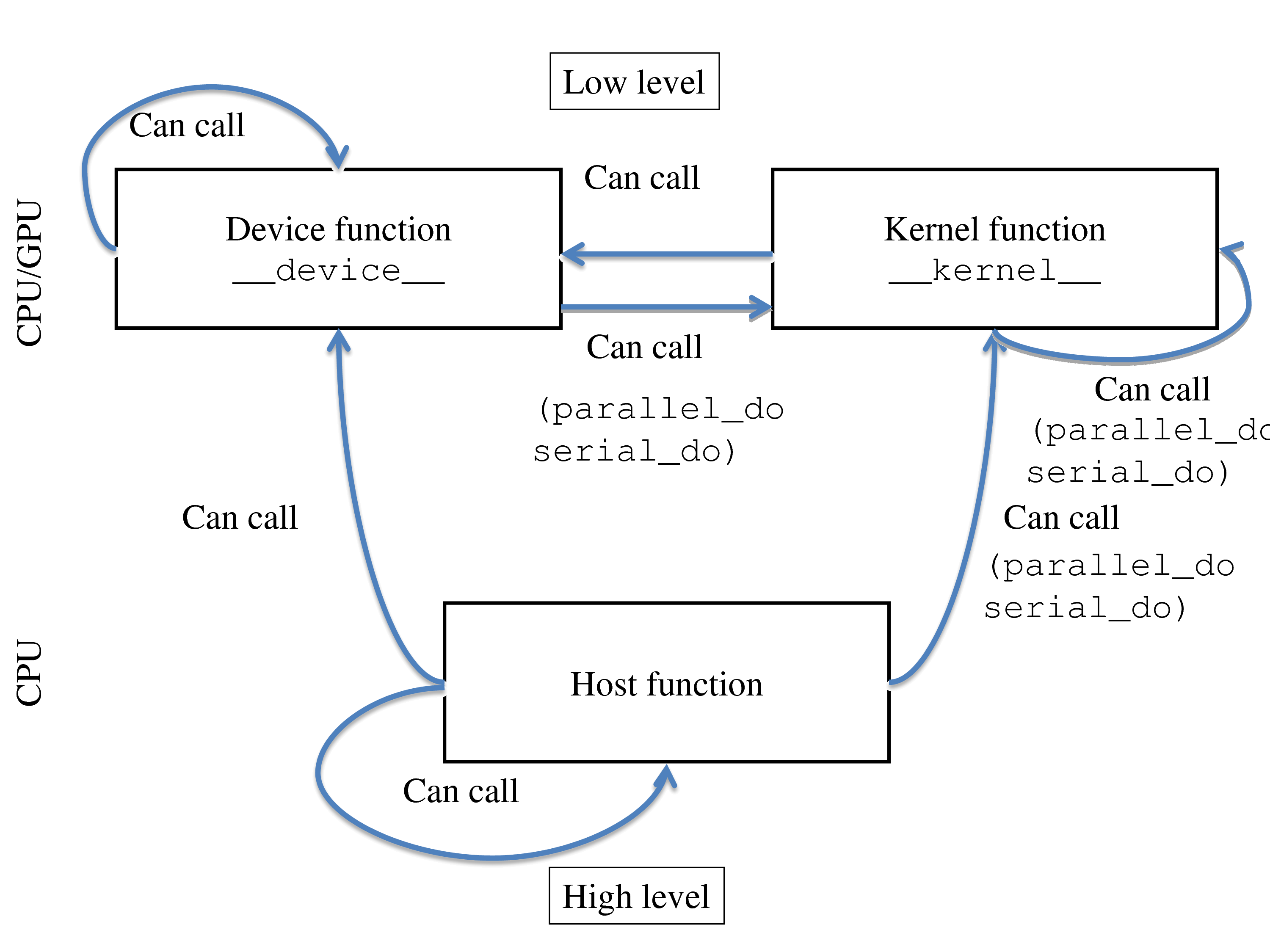
As already mentioned in Section 2.4↑, there are three types of functions in Quasar: device functions, kernel functions and host functions. There are strict rules about how functions of a different type can call each other:
- Both __kernel__ and __device__ functions are low-level functions, they are natively compiled for CPU and/or GPU. This has the practical consequence that the functionality available for these functions is restricted. It is for example not possible to load or save information inside kernel or device functions. On the contrary, the print function is supported, but only for string, scalar, int, cscalar, vecX, ivecX and cvecX datatypes.
- Host functions are high-level functions, typically they are interpreted (or Quasar EXE’s, compiled using the just-in-time compiler).
- A kernel function is normally repeated for every element of a matrix. Kernel functions can only be called using the parallel_do/serial_do functions.
- A device function can be called from host code or from other device/kernel functions.
- Kernel and device functions can call other kernel functions, through parallel_do/serial_do (nested parallelism, see Section 4.4↓).
The distinction between these three types of functions is necessary to allow GPU programming. Furthermore, it provides a mechanism to balance the work between CPU/GPU. To find out whether the code will be run on GPU/CPU, the following recipe can be used:
- Kernel functions are a candidate to run on the GPU. When the kernel function is sufficiently “heavy” (i.e. data dimensions ≥ 1024, branches, thread synchronization), there is a high likelihood that the function will be executed on the GPU.
- Device functions run on the GPU (when called from a kernel function that is launched on the GPU) or on the CPU.
- Host functions run exclusively on the CPU.
4.4 Nested parallelism
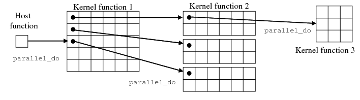
__kernel__ and __device__ functions can also launch nested kernel functions using the parallel_do (and serial_do) functions. The top-level host function may for example launch 30 threads (see Figure 4.2↓), from which every of these 30 threads spans again 12 threads (after some algorithm-specific initialization steps). There are several advantages of this approach:
- More flexibility in expressing the algorithms
- The nested kernel functions are mapped onto CUDA dynamic parallelism on Kepler devices such as the Geforce GTX 780, Geforce GTX Titan or newer.
- When a parallel_do is placed inside a __device__ function that is called directly from the host code (CPU computation device), the parallel_do will be accelerated using OpenMP.
Notes:
- There is no guarantee that the CPU/GPU will effectively perform the nested operations in parallel. However, future GPUs may be expected to become more efficient in handling parallelism on different levels.
- The setting “dynamic parallelism” needs to be enabled. By default, inner kernels are executed sequentially.
Limitations:
- Nested kernel functions may not use shared memory (they can access the shared memory through the calling function however), texture memory, and they may also not use thread synchronization.
- Currently only one built-in parameter for the nested kernel functions is supported: pos (and not blkpos, blkidx or blkdim).
In fact, when nesting parallel_do and serial_do and considering two levels of nesting, there are four possibilities:
| Outer operation | Inner operation | Result |
| serial_do | serial_do | Sequential execution on CPU |
| serial_do | parallel_do | Parallel execution on CPU via OpenMP |
| parallel_do | serial_do | Execution on GPU, inner kernel is executed sequentially |
| parallel_do | parallel_do | Execution on GPU, sequentially (default) or CUDA dynamic parallelism (when enabled) |
4.5 Function overloading
To implement functions taking different argument with different types, the most simple approach is to check the types of the function at runtime. Consider for example the following function that computes the Hermitian transpose of a matrix:
function y = herm_transpose(x:[scalar|cscalar|mat|cmat])
if isscalar(x)
y = conj(x)
elseif isreal(x)
y = transpose(x)
elseif iscomplex(x)
y = conj(transpose(x))
endif
endfunction
Although this technique is legal in Quasar, it has two important disadvantages:
if isscalar(x)
y = conj(x)
elseif isreal(x)
y = transpose(x)
elseif iscomplex(x)
y = conj(transpose(x))
endif
endfunction
- Type inference is difficult: the compiler cannot uniquely determine the type of the result of herm_transpose(x), because the type depends on the type of x (and the conditions used in the if clauses). Instead, the compiler will assume that the resulting type is unknown (‘??’). Hence, several optimizations (such as loop parallelization) that apply to code blocks that make use of the result of herm_transpose(x), will be disabled.
- Runtime checking of variable types creates some additional overhead, while in this case this could be handled perfectly by the compiler.
For these reasons, Quasar supports function overloading. The above function could be implemented as follows:
function y = herm_transpose(x : cscalar)
y = conj(x)
endfunction
function y = herm_transpose(x : scalar)
y = x
endfunction
function y = herm_transpose(x : mat)
y = transpose(x)
endfunction
function y = herm_transpose(x : cmat)
y = conj(transpose(x))
endfunction
y = conj(x)
endfunction
function y = herm_transpose(x : scalar)
y = x
endfunction
function y = herm_transpose(x : mat)
y = transpose(x)
endfunction
function y = herm_transpose(x : cmat)
y = conj(transpose(x))
endfunction
In case none of the definitions apply, the compiler will generate an error stating that the function herm_transpose is not defined for the given input variable types. The overload resolution (i.e. the method the compiler uses for selecting the correct overload), follows the rules of the reduction resolution, which will be discussed in Section 4.9↓.
Note that the function overloading has the following restrictions:
- all function overloads must reside within the same module.
- all function overloads must be defined at the global scope (i.e. not inside another functions).
- only host and device functions can be overloaded, not __kernel__ functions or lambda expressions.
- function overloads must differ in number of input arguments (or input argument types). Thereby, differences in output arguments are ignored.
- it is not possible to obtain a function handle of an overloaded function. Internally, overloaded functions are converted by the compiler to reductions (see Section 4.9↓).
Finally, when the type of the input variables is not known to the compiler, the overload resolution will be performed at runtime.
4.5.1 Device function overloading
Some functions, especially functions from the standard libraries, are often used in different circumstances:
- within a host function, e.g., to process one single huge matrix
- from a kernel/device function, where the function is to be executed with many threads in parallel.
One notable example is the svd (singular value decomposition) function: when called from a device function, svd needs to be specialized for small matrices, while in a host function, svd may need to deal with large matrices (resulting in entirely different parallel implementations). Therefore, the host function can be overloaded using a device function with exactly the same signature (apart from the __device__ specifier):
function [p:mat,d:mat,q:mat] = svd(a:mat)
...
endfunction
function [p:mat,d:mat,q:mat] = __device__ svd(a:mat)
...
endfunction
...
endfunction
function [p:mat,d:mat,q:mat] = __device__ svd(a:mat)
...
endfunction
when svd is then user from a kernel/device function, the device overload is used. On the other hand, when called from a host function, the host overload will be used. In case only a device function is provided (and no host function overload), then the device function can also still be called from the host function (see Figure 4.1↑) but then it is not possible to have different implementations.
Overloading is possible for size and dimension constraints (see 3.4↑). This allows the svd function to be overloaded for 2 × 2 matrices:
function [p:mat2x2,d:mat2x2,q:mat2x2] = __device__ svd(a:mat2x2)
...
endfunction
The compiler then exploits the available type information to find the most efficient implementation for the given type.
...
endfunction
4.5.2 Optional function parameters
It is possible to declare values for optional function parameters. When the parameter is not used, the specified default value is used. For example,
function y = func1(x = eye(4))
function y = func2(x = eye(4), y = [[1,2],[3,4]])
function y = func2(x = eye(4), y = [[1,2],[3,4]])
func1() % same as func1(eye(4))
func1(eye(5))
func2(x:=eye(3), y:=randn(6))
func2(y:=4)
Named optional parameters can be specified through the x:=value syntax. This is mainly useful when for example the first optional argument will be omitted, but not the second.
func1(eye(5))
func2(x:=eye(3), y:=randn(6))
func2(y:=4)
As indicated in the above example, the optional values can be expressions. These expressions are evaluated when the function is called and when no argument is used. It is recommended to only use functions with no other side effects other than calculating the value of the optional parameter. The expressions may refer to other parameters, but only in the order that the parameters are passed:
function y = func3(x, y = 3*x)func3(eye(4))Here, by default y = 3*eye(4), will be used.
4.6 Functions versus lambda expressions
In Quasar, a function is defined as follows:
function y = fused_multiply_add(a, b, c)
y = a * b + c
endfunction
On the other hand, a lambda expression can be defined to compute the same result:fused_multiply_add = (a, b, c) -> a * b + cThe question is then: what is the difference between functions and lambda expressions apart from their syntax? From a run-time perspective, lambda expressions and functions are treated in the same way in Quasar: both are functions of type (??,??,??) -> ??. The difference is only visible at compile-time:
y = a * b + c
endfunction
- Functions can have optional arguments, whereas lambda expressions cannot.
- Functions are named, while lambda expressions are often anonymous.
- Functions can be overloaded (see Section 4.5↑), in contrast to lambda expressions, which can not be overloaded. A second definition with the same name simply overwrites the first definition; moreover, the function variable may become polymorphic.
- Both functions and lambda expressions can have multiple output arguments. For lambda expressions, this requires the variable to be explicitly typed (see Subsection 4.6.1↓).
- Both functions and lambda expressions can have closures (see Section 4.2↑).
- Lambda expressions can have block statements (aa; bb; cc); although they cannot contain control structures (if, for, while, etc.)
On the other hand, the definition of lambda expressions is more compact, and lambda expressions are often inlined by default by the compiler.
Hence, the programmer may choose whether a function is preferable for a given situation, or a lambda expression. A summary of the resemblances and differences between functions and lambda expressions is given in Table 4.1↓.
Table 4.1 Comparison of functions and lambda expressions
| Function | Lambda expression | |
| Optional arguments | Yes | No |
| Multiple output arguments | Yes | Yes |
| Supports overloading | Yes | No |
| __kernel__, __device__ | Yes | Yes |
| Function closures | Yes | Yes |
| Function handles ((??,??)->??) | Yes | Yes |
| First-class citizen | Yes | Yes |
| Can contain control structures | Yes | No |
| Can contain nested functions | Yes | No |
| Can contain nested lambda expressions | Yes | Yes |
4.6.1 Explicitly typed lambda expressions
A lambda expression can either be partially typed or explicitly typed. In the former case, the type of the lambda expression parameters are typed, which causes the return value of the lambda expression to be determined by type inference:
sincos = (x : scalar) -> [sin(x), cos(x)]In the latter case, the variable capturing the lambda expression is explicitly typed:
sincos : [scalar -> (scalar, scalar)] =
x -> {sin(x), cos(x)}
This syntax has two benefits:
x -> {sin(x), cos(x)}
- Lambda expressions with multiple output arguments can be defined. Whereas in the first example, the lambda expression returns a single output argument, i.e., vector of length two, in the second example, the lambda expression itself has two output arguments.
-
The explicit type is applied recursively to inner lambda expressions. For example, the higher-level lambda expression (see Section 4.10↓):add : [scalar->scalar->scalar] = x -> y -> x + yis equivalent to:add : (x : scalar) -> (y : scalar) -> x + yWhen the explicit type is subsequently replaced by type alias, multiple lambda expressions can share the same signature:type binary_op : [scalar -> scalar -> scalar]
add : binary_op = x -> y -> x + y
sub : binary_op = x -> y -> x - y
Explicitly typed lambda expressions will be further used in the section on functional programming in Quasar (see Chapter 15↓).
4.7 Kernel function output arguments
To improve the syntax for kernel functions that have scalar output variables (e.g., sum, mean, standard deviation, ...), kernel output arguments are added as a special language feature to Quasar. The feature is special, because kernel functions intrinsically generate multiple output values, as they are applied to a typically large number of elements, while here there is only one value per output argument. The kernel output arguments are shared between all threads and all blocks. Moreover, the kernel output arguments are restricted to be of the type scalar, cscalar, int, ivecX, vecX and cvecX. The following example illustrates the use of kernel function output arguments:
function [y : int] = __kernel__ any(A : mat, pos : ivec2)
if A[pos] != 0
y = 1
endif
endfunction
if parallel_do(size(A),A,any)
print "At least one element of A is non-zero!"
endif
if A[pos] != 0
y = 1
endif
endfunction
if parallel_do(size(A),A,any)
print "At least one element of A is non-zero!"
endif
The function any returns 1 when at least one element of the input matrix A is nonzero. The variable y is initialized by zero by the parallel_do function, before the first call to any is made.
Kernel function output arguments are also subject to data races (see Subsection 2.4.4↑), therefore atomic operations should be used! Remark that atomic operations also cause some overhead, and are only useful when there are only a small number of writes to the output arguments. In the following example, the sum of the elements of a sparse matrix A is computed.
function [sum : scalar] =
__kernel__ stats(A : mat, pos : ivec2)
if A[pos] != 0
sum += A[pos]
endif
endfunction
sum = parallel_do(size(A),A,stats)
__kernel__ stats(A : mat, pos : ivec2)
if A[pos] != 0
sum += A[pos]
endif
endfunction
sum = parallel_do(size(A),A,stats)
This output argument accumulation approach is only recommended when the number of nonzero elements of A is small compared to the total number of elements of A (lets say, less than 1%). In other cases, implementation of the sum using parallel reductions (see Section 10.6↓) is more efficient!
After completion of the kernel function, the output arguments of the kernel function are directly copied back to the CPU memory. This may not be desirable because this creates an implicit device-host synchronization point. For multi-GPU processing (see 11↓), this may cause one or multiple GPUs to become idle. The solution in this case is to use input parameters instead of output parameters:
function [] = __kernel__ stats(sum : vec(1), A : mat, pos : ivec2)
if A[pos] != 0
sum[0] += A[pos]
endif
endfunction
sum = zeros(1)
parallel_do(size(A),sum,A,stats)
The result is here stored in the vector sum. Only at the moment that the exact value of sum is needed (e.g., when evaluating sum[0]), a memory transfer and synchronization between GPU and CPU. This can be avoided in case a subsequently launched kernel function directly reads sum[0] via the device memory.
if A[pos] != 0
sum[0] += A[pos]
endif
endfunction
sum = zeros(1)
parallel_do(size(A),sum,A,stats)
4.8 Variadic functions
Variadic functions are functions that can have a variable number of arguments. For example:
function [] = func(... args)
for i=0..numel(args)-1
print args[i]
endfor
endfunction
func(1, 2, "hello")
for i=0..numel(args)-1
print args[i]
endfor
endfunction
func(1, 2, "hello")
Here, args is called a rest parameter (which is similar to ECMAScript 6). How does this work: when the function func is called, all arguments are packed in a cell vector which is passed to the function. Optionally, it is possible to specify the types of the arguments:
function [] = func(... args:vec[string])
which indicates that every argument must be a string, so that the resulting cell vector is a vector of strings.
Several library functions in Quasar already support variadic arguments (e.g. print, plot, \SpecialChar ldots), although now it is possible to define your own functions with variadic arguments.
Moreover, a function may have a set of fixed function parameters, optional function parameters and variadic parameters. The variadic parameters should always appear at the end of the function list (otherwise a compiler error will be generated)
function [] = func(a, b, opt1=1.0, opt2=2.0, ...args)
endfunction
endfunction
This way, the caller of func can specify extra arguments when desired. This allows adding extra options for e.g., solvers.
4.8.1 Variadic device functions
It is also possible to define device functions supporting variadic arguments. These functions will be translated by the back-end compilers to use cell vectors with dynamically allocated memory (it is useful to consider that this may have a small performance cost).
An example:
function sum = __device__ mysum(... args:vec)
sum = 0.0
for i=0..numel(args)-1
sum += args[i]
endfor
endfunction
sum = 0.0
for i=0..numel(args)-1
sum += args[i]
endfor
endfunction
function [] = __kernel__ mykernel(y : vec, pos : int)
y[pos]= mysum(11.0, 2.0, 3.0, 4.0)
endfunction
y[pos]= mysum(11.0, 2.0, 3.0, 4.0)
endfunction
Note that variadic kernel functions are not supported.
4.8.2 Variadic function types
Variadic function types can be specified as follows:
fn : [(...??) -> ()]
fn2 : [(scalar, ...vec[scalar]) -> ()]
fn2 : [(scalar, ...vec[scalar]) -> ()]
This way, functions can be declared that expect variadic functions:
function [] = helper(custom_print : [(...??) -> ()])
custom_print("Stage", 1)
...
custom_print("Stage", 2)
endfunction
custom_print("Stage", 1)
...
custom_print("Stage", 2)
endfunction
function [] = myprint(...args)
for i=0..numel(args)-1
fprintf(f, "%s", args[i])
endfor
endfunction
helper(myprint)
for i=0..numel(args)-1
fprintf(f, "%s", args[i])
endfor
endfunction
4.8.3 The spread operator
The spread operator unpacks one-dimensional vectors, allowing them to be used as function arguments or array indexers. For example:
pos = [1, 2]
x = im[...pos, 0]
x = im[...pos, 0]
In the last line, the vector pos is unpacked to [pos[0], pos[1]], so that the last line is in fact equivalent with
x = im[pos[0], pos[1], 0]
Note that the spread syntax ... makes the writing of the indexing operation a lot more convenient. An additional advantage is that the spread operator can be used, without knowing the length of the vector pos. Assume that you have a kernel function in which the dimension is not specified:
function [] = __kernel__ colortransform (X, Y, pos)
Y[...pos, 0..2] = RGB2YUV(Y[...pos, 0..2])
endfunction
This way, the colortransform can be applied to a 2D RGB image, as well as a 3D RGB image. Similarly, if you have a function taking three arguments, such as:
Y[...pos, 0..2] = RGB2YUV(Y[...pos, 0..2])
endfunction
luminance = (R,G,B) -> 0.2126 * R + 0.7152 * G + 0.0722 * BThen, typically, to pass an RGB vector c to the function luminance, you would use:
c = [128, 42, 96]
luminance(c[0],c[1],c[2])
Using the spread operator, this can simply be done as follows:
luminance(c[0],c[1],c[2])
luminance(...c)
The spread operator also has a role when passing arguments to functions. Consider the following function which returns two output values:
function [a,b] = swap(A,B)
[a,b] = [B,A]
endfunction
[a,b] = [B,A]
endfunction
And we wish to pass both output values to one function
function [] = process(a, b)
...
endfunction
...
endfunction
Then using the spread operator, this can be done in one line:
process(...swap(A,B))
Here, the multiple values [a,b] are unpacked before they are passed to the function process. This feature is particularly useful in combination with variadic functions.
Notes:
- Only vectors (i.e., with dimension 1) can currently be unpacked using the spread operator. This may change in the future.
- Within kernel/device functions, the spread operator is currently supported on vector types vecX, cvecX, ivecX (this means: the compiler should be able to statically determine the length of the vector).
- Within host functions, cell vectors can be unpacked as well.
-
The spread operator can be used for concatenating vectors and scalars:a = [1,2,3,4]where c will be a vector of length 8. For small vectors, this is certainly a good approach. For long vectors, this technique may have a poor performance, due to the concatenation being performed on the CPU. In the future, the automatic kernel generator may be extended, to generate efficient kernel functions for the concatenation.
b = [6,7,8]
c = [...a, 4, ...b]
4.8.4 Variadic output parameters
The output parameter list does not support the variadic syntax .... Instead, it is possible to return a cell vector of a variable length.
function [args] = func_returning_variadicargs()
args = vec[??](10)
args[0] = ...
endfunction
The resulting values can then be captured in the standard way as output parameters:
args = vec[??](10)
args[0] = ...
endfunction
a = func_returning_variadicargs() % Captures the cell vector
[a] = func_variadicargs() % Captures the first element, and generates an
% error if more than one element is returned
[a, b] = func_variadicargs() % Captures the first and second elements and
% generates an error if more than one element
% is returned
Additionally, using the spread operator, the output parameter list can be unpacked and passed to any function:
[a] = func_variadicargs() % Captures the first element, and generates an
% error if more than one element is returned
[a, b] = func_variadicargs() % Captures the first and second elements and
% generates an error if more than one element
% is returned
myprint(...func_variadicargs())
4.9 Reductions
Quasar implements a very flexible compile-time graph reduction scheme to allow expression transformations. Reductions are defined inside Quasar programs through a special syntax and allow the compiler to “reason” about the operations being performed in the program, without having to evaluate these operations. The syntax is as follows:
reduction (var1:t1, ..., varN:tN) -> expr(var1,...,varN) = substitute(var1,...,varN)
Once the reduction has been defined, the compiler will attempt to apply the reduction each time an expression that matches with expr has been found. Expressions can be regular Quasar expressions and are not restricted to functions. For example, suppose that we have an efficient implementation for the fused multiply-add operation a+b*c, called fmad(a,b,c), we can use this implementation for all combinations a+b*c that occur in the program. This is achieved by defining the following reduction:
reduction (a:cube, b:cube, c:scalar) -> a+b*c = fmad(a,b,c) _
where size(a) == size(b)
Remark that we explicitly indicated the types of the variables a,b and c for which this reduction is applicable, together with a restriction on the sizes of a and b (size(a) == size(b)).
where size(a) == size(b)
Reductions can also be used to define an alternative implementation for a cascade of functions:
reduction (x) -> real(ifft2(x)) = irealfft2(x)Here, a complex->real (C2R) 2D FFT algorithm (implemented by irealfft2(x)) will be used to compute real(ifft2(x)). Because the C2R FFT operates on half the amount of memory of a complex->complex (C2C) FFT, the performance will be increased by roughly a factor of two!
Reductions are also ideal for some clever “trivial” optimizations:
reduction (x:mat) -> real(x) = x
reduction (x:mat) -> imag(x) = zeros(size(x))
reduction (x:mat) -> transpose(transpose(x)) = x
reduction (x:mat) -> x[:,:] = x
reduction (x:mat) -> real(transpose(x)) = transpose(real(x))
reduction (x:mat) -> imag(x) = zeros(size(x))
reduction (x:mat) -> transpose(transpose(x)) = x
reduction (x:mat) -> x[:,:] = x
reduction (x:mat) -> real(transpose(x)) = transpose(real(x))
Using the above reductions, the compiler will simplify the following expression:
f = (x : mat) -> transpose(real(ifft2(fft2(transpose(x)))))
as follows:
Applied reduction ifft2(fft2(transpose(x))) -> transpose(x)
Applied reduction real(transpose(x)) -> transpose(x)
Applied reduction (x:mat) -> transpose(transpose(x)) -> x
Result after 3 reductions: f=(x:mat) -> x
Applied reduction real(transpose(x)) -> transpose(x)
Applied reduction (x:mat) -> transpose(transpose(x)) -> x
Result after 3 reductions: f=(x:mat) -> x
Hence, the compiler finds that the operation f(x) is an identity operation! In this trivial example, we can assume that the programmer would have found the same result, however there are some situations that we will describe later in this section, in which the reduction technique can save a lot of time for the programmer.
Clearly, reductions bring the following benefits:
- Define once, optimal everywhere!
- More readable and clean optimized code compared to other programming languages that do not use reductions.
- The compiler can indicate some places in the code suited for optimization, but where e.g., some of the types of the variables is not known.
To avoid typing the same reduction with different types over and over again, type classes can be used (see Section 3.7↑):
type RealNumber: [scalar|cube|AllInt|cube[AllInt]]
type ComplexNumber: [cscalar|ccube]
reduction (x : RealNumber) -> real(x) = x
reduction (x : ComplexNumber) -> complex(x) = x
Without type classes, the reduction would need to be written four times.
type ComplexNumber: [cscalar|ccube]
reduction (x : RealNumber) -> real(x) = x
reduction (x : ComplexNumber) -> complex(x) = x
4.9.1 Symbolic variables and reductions
A special subset of the reductions are the symbolic reductions. Symbolic reductions often operate on variables that are “not defined” using the regular variable semantics. An example is given below:
reduction (x : scalar, a : scalar) -> diff(a, x) = 0
reduction (x : scalar, a : int) -> diff(x^a,x) = a*x^(a-1)
reduction (x, y, z : scalar) -> diff(x + y, z) = diff(x, z) + diff(y, z)
reduction (x : scalar, y : scalar) -> diff(x, y) = 0
reduction (x, y : scalar) -> diff(sin(x),y) = cos(x) * diff(x, y)
f = x -> diff(sin(x^4)+2,x) % Simplifies to 4*cos(x^4)*x^3
reduction (x : scalar, a : int) -> diff(x^a,x) = a*x^(a-1)
reduction (x, y, z : scalar) -> diff(x + y, z) = diff(x, z) + diff(y, z)
reduction (x : scalar, y : scalar) -> diff(x, y) = 0
reduction (x, y : scalar) -> diff(sin(x),y) = cos(x) * diff(x, y)
To be able to calculate derivatives with respect to variables that have not been defined/initialized, symbolic variables can be used, using the symbolic keyword:symbolic x : int, y : scalar
These variables have no further meaning during the execution of the program. As such, during runtime, they do not exist. However, they help writing symbolic expressions:
reduction (f, x : scalar) -> argmin(f, x) = solve(diff(f, x) = 0, x)
symbolic x : scalar
print argmin((x-2)^2, x)
symbolic x : scalar
print argmin((x-2)^2, x)
Here, the definition of x as a symbolic scalar is required, otherwise the compiler would not have any type information about x. Then, in case the compiler is not able to determine the minimum argmin, an error will be generated:
Line 3: Symbolic operation failed - no reductions available for ’argmin((x-2)^2, x)’
4.9.2 Reduction resolution
This subsection describes how Quasar decides which reduction to use at a particular time, and also in which order several reductions need to be applied. Suppose that we have an expression like:
reduction (A : mat, x : vec’col) -> A*x = f(x) % RED #1
reduction (A : mat, B : mat) -> norm(A, B) = sum((A-B).^2) % RED #2
g = (x : vec’col, b : vec’col) -> norm(A*x, b)
reduction (A : mat, B : mat) -> norm(A, B) = sum((A-B).^2) % RED #2
g = (x : vec’col, b : vec’col) -> norm(A*x, b)
Then, both RED#1 and RED#2 can be applied. Quasar will prioritize reductions that have larger number of input variables (in this case RED#2, with input variables A and B). Reductions that having more variables are generally more difficult to match (because they contain more conditions that need to be satisfied than reductions with for example 1 variable). Moreover, it is assumed that, in terms of expression optimization, reductions with more variables are designed to be more efficient. Therefore, the reduction will proceed as follows:
g = x -> sum((A*x-b).^2)
g = x -> sum((f(x)-b).^2)
g = x -> sum((f(x)-b).^2)
In this case, the result is actually independent of the order of reduction application. However, there are cases where the order make play a role, such that the end result may differ. This is called a reduction conflict. Reduction conflicts will be further treated in Subsection 4.9.3↓.
When the number of variables of two reductions is equal. Another criterion is needed to decide which reduction needs to be applied first. Quasar currently uses a three-level decision rule:
- Prioritize reductions with the largest numbers of variables.
- Prioritize exact matches. For example, A:vec may match a reduction with variables (x:mat), because vec ⊂ mat (see Section 2.2↑). However, when a reduction exists that has as input x:vec, this reduction will be prioritized.
-
Prioritize application to expressions with a higher depth in the expression tree representation. Sometimes the same reduction may be applied twice within the same expression. For example, inreduction x -> sum(x) = my_sum(x)the sum reduction can be applied twice. The order is then from right to left, which enables correct type inference (the reduction to apply for the second step may depend on the type of my_sum(x). In terms of an expression tree representation, this comes down to prioritizing applications with a higher depth in the expression tree (root=depth 0, children=depth 1, ...). Hence, the reduction proceeds as follows:
f = x -> sum(sum(x))f = x -> sum(my_sum(x))
f = x -> my_sum(my_sum(x))
By these rules, the reduction application will work as “expected”, and also for function applications (see Section 4.5↑). Overloaded functions are in fact internally implemented in Quasar using reductions:
reduction (x : cscalar) -> herm_transpose(x) = herm_transpose_cscalar(x)
reduction (x : scalar) -> herm_transpose(x) = herm_transpose_scalar(x)
reduction (x : mat) -> herm_transpose(x) = herm_transpose_mat(x)
reduction (x : cmat) -> herm_transpose(x) = herm_transpose_cmat(x)
reduction (x : scalar) -> herm_transpose(x) = herm_transpose_scalar(x)
reduction (x : mat) -> herm_transpose(x) = herm_transpose_mat(x)
reduction (x : cmat) -> herm_transpose(x) = herm_transpose_cmat(x)
4.9.3 Ensuring safe reductions
If not used correctly, reductions may introduce errors (bugs) in the Quasar program that may be difficult to spot. To prevent this from happening, the Quasar compiler detects a number of situations in which the application of a reduction is considered to be unsafe. The reduction safety level can be configured using the COMPILER_REDUCTION_SAFETYLEVEL variable (see Table 17.3↓). This variable can take the following values:
- NONE: perform no safety checks
- SAFE: perform safety checks and report a warning in case of a problem
- STRICT: generate an error in case “unsafe” reductions have been detected.
There are five situations in which a reduction is considered to be unsafe:
- Free variables in reduction: the right handed side of the reduction contains a variable that is not present in the left handed side. For example:reduction x -> f(x) + yHere the variable y causes a problem because the compiler does not have any information on this variable. It is hence unbound. The problem can be fixed in this case:reduction (x, y) -> f(x) + y
- Undefined functions in reductions: all functions in the right handed side of the reduction need to be defined in Quasar, either through standard definitions, or through other reductions.
-
Reduction operands defined in non-local scope: when some of the operands to which a reduction is applied to, are defined in a non-local context, side-effects maybe created in case these non-local variables are modified afterwards. For example, a change of type may cause the reduction application to be invalid at run-time, even though it seemed valid at compile-time. For example:reduction x:mat -> ifft2(fft2(x)) = x
A = ones(4,4)
for k=1..10
y = x:mat -> ifft2(fft2(x + A))
A = load("myfile.dat") # may cause the reduction
# ifft2(fft2(x))=x to be invalid.
endfor -
Reduction conflicts: sometimes, the result of the application of several reductions may depend on the order of the reductions. Usually, this is a result of poor definitions of the reductions, as demonstrated in the following example:reduction (A : mat, B : mat, x : vec’row) -> norm(A*x, B) = f(A, B, x) % RED #1In this example, we could either apply reduction #1 or reduction #2. According to the reduction resolution results (see Subsection 4.9.2↑), the Quasar compiler will choose reduction #1 because it has three variables, A, B and x. However, applying reduction #2 would result in a completely different result sum((A*x-B).^2) and it is not guaranteed that f(A, B, x)=sum((A*x-B).^2). The compiler detects this automatically and raises the reduction conflict error/warning whenever there is a problem. Here, the reduction conflict can be solved by defining:reduction (A : mat, B : mat, x : vec’row) -> f(A, B, x) = sum((A*x-B).^2)
reduction (A : mat, B : mat) -> norm(A, B) = sum((A-B).^2) % RED #2
g = (x : vec’row, b : vec’row) -> norm(A*x, b) -
Reduction cross-references: circular dependencies may be created between reductions:reduction (A, B) -> f(A, B) = g(A, B)This obviously is also not allowed and will generate a compiler error.
reduction (A, B) -> g(A, B) = f(A, B)
These rules allow to write safe Quasar reductions which cause no undesired side-effects.
4.9.4 Reduction where clauses
Reductions can also be applied in a conditional way. This is achieved by specifying a where clause. The where clause determines at compile time (or at runtime) whether a given reduction may be applied. There are two main use cases for where clauses:
- To avoid invalid results: In some circumstances, applying certain reductions may lead to invalid results (for example a real-valued sqrt function applied to a complex-valued input, derivative of tan(x) in π ⁄ 2\SpecialChar ldots)
- For optimization purposes (e.g. allowing alternative calculation paths).
For example:
reduction (x : scalar) -> abs(x) = x where x >= 0 reduction (x : scalar) -> abs(x) = -x where x < 0 In case the compiler has no information on the sign of x, the following mapping is applied:
abs(x) -> x >= 0 ? x : (x < 0 ? -x : abs(x))
And the evaluation of the where clauses of the reduction is performed at runtime.
However, when the compiler has information on x (e.g. assert(x = -1)), the mapping will be much simpler:
However, when the compiler has information on x (e.g. assert(x = -1)), the mapping will be much simpler:
abs(x) -> -x
Note that the abs(.) function is a trivial example, in practice this could be more complicated:
reduction (x : scalar) -> someop(x, a) = superfastop(x, a) where 0 <= a && a < 1
reduction (x : scalar) -> someop(x, a) = accurateop(x, a) where 1 <= a
reduction (x : scalar) -> someop(x, a) = accurateop(x, a) where 1 <= a
There are also three special conditions that can be used inside reductions. These conditions are mainly used internally by the Quasar compiler, but can also be useful for certain user optimizations:
- $ftype("__host__"): is true only when the outer function is a host (i.e. non-kernel/device function)
- $ftype("__device__"): is true only when the outer function is a device function
- $ftype("__kernel__"): is true only when the outer function is a device function
These conditions reduce the applicability of the reduction depending on the outer function scope in which the reduction is to be applied. For example, it is possible to specify reductions that can only be used inside device functions, reductions for host functions etc.
4.9.5 Variadic reductions
In analogy to variadic functions (see 4.8↑), it is possible to define reductions with a variable number of arguments. The main use of variadic reductions is two-fold:
- Providing a calling interface to variadic functions:reduction (a : string, ...args : vec[??]) -> myprint(a, args) = handler(a, ...args)This avoids defining several reductions (one reduction for n number of parameters) in order to call variadic functions.
-
Capturing symbolic expressions with variable number of terms. Suppose that we want to define a reduction for the following expression:λ1(f1(x))2 + λ2(f2(x))2 + ... + λK(fK(x))2where f1, f2, ..., fK are functions to be captured, λ1, λ2, ..., λK are scaling parameters and where the number of terms K is variable. A reduction for this expression can be defined as follows:reduction (x, ...lambda, ...f) -> sum([lambda*f(x).^2]) = mysum(f,lambda)Here, lambda and f are variadic captures, their type is a cell vector of respectively scalars and functions (i.e., vec and vec[[??->??]]). Such reduction can match expressions like:2*(x.^2) + cos(3)*((2*x).^2) + 2*((-x).^2)
4.10 Partial evaluation
Quasar has a complete implementation of lambda expressions, and also allows partial evaluation:
f = (x, y) -> x + y
g = y -> x -> f(x, y)
print g(4)(5) % Will return 9
g = y -> x -> f(x, y)
print g(4)(5) % Will return 9
Here, the partial evaluation x -> f(x, y), returns a lambda expression that adds the free variable y to its input, x. Consider for example a linear solver, that solves Ax = y, using the function x=lsolve(A, y). Suppose that we have a large number of linear systems that need to be solved. Then we can define the partial evaluation of lsolve:
lsolver = A -> y -> lsolve(A, y)
solver = lsolver(A)
for k=1..100
x[k] = solver(y[k])
endfor
solver = lsolver(A)
for k=1..100
x[k] = solver(y[k])
endfor
Similarly, we can have a lambda expression that solves a quadratic equation Ax2 + Bx + C = y: x=qsolve(A, B, C - y), by returning for example the largest solution:
qsolver = (A, B, C) -> y -> qsolve(A, B, C - y)
solver = qsolver(A, B, C)
for k=1..100
x[k] = solver(y[k])
endfor
solver = qsolver(A, B, C)
for k=1..100
x[k] = solver(y[k])
endfor
Now, solver(y) is a generic solver that can be used in other numerical techniques, while lsolver and qsolver can be used to create the desired solver.
It is also possible to define lambda expressions that have another lambda expression as input. The syntax is not f = (x -> y) -> g(x), but:h = (x : lambda_expr) -> f(x(y))
or, more type-safe versions:
h = (x : [?? -> ??]) -> f(x(y))
h = (x : [cube -> cube]) -> f(x(y))
h = (x : [cube -> cube]) -> f(x(y))
For example, we can define a lambda expression that sums the output of two other lambda expressions f1 and f2, again as another lambda expression:f = (f1 : [?? -> ??], f2 : [?? -> ??]) = x -> f1(x) + f2(x)
or, even more generally, using reductions:
reduction (f1 : [?? -> ??], f2 : [?? -> ??], x) -> f1 + f2 = x -> f1(x) + f2(x)
f1 = x -> x * 2
f2 = x -> x / 2
f3 = f1 + f2 % Result: f3 = x -> x * 2 + x / 2
f1 = x -> x * 2
f2 = x -> x / 2
f3 = f1 + f2 % Result: f3 = x -> x * 2 + x / 2
Recursive lambda expressions can be defined simply as:
factorial = (x : scalar) -> (x > 0) ? x * factorial(x - 1) : 1
One only needs to be careful that the recursion stops at a given point (otherwise a stack overflow error will be generated [I] [I] Note: tail recursion optimization is currently not supported, however, for device lambda functions the underlying back-end compiler may perform this optimization.).
4.11 Code attributes
Code attributes provide a means to incorporate meta-data in Quasar source code files. Additionally, code attributes also allow passing information to the compiler and runtime systems.
The general syntax of a code attribute is as follows:
{!attribute prop1=value1, ..., propN=valueN}
where attribute is the name of the code attribute, prop1 and propN are parameter names and value1 and valueN are the respective values.
The following code attributes are currently available:
-
Annotation data:
Code attribute Purpose {!author name="" } Adds the name of the author to the source file. Multiple authors can be specified using a comma-separated list {!doc category=""} The category of the module in the documentation system {!copyright text=""} A copyright text for the current source code file {!description text=""} A brief description of the purpose of the source code file {!region name=""} Begins a region in the source code (which is automatically folded by the editor) {!endregion} Ends a region in the source code -
Compiler code attributes:
Code attribute Purpose {!auto_inline} Automatically inlines the current function {!auto_vectorize} Automatically vectorizes code within the current block {!specialize args=(arglist)} Automatically specializes a function based on the specified argument list {!kernel target="cpu|gpu|..."} Sets the target of the kernel function (see Subsection 17.2.5↓) {!kernel_transform Enables a given kernel transform enable="(transform)"} {!kernel_arg name=arg} Annotates kernel arguments with data that can be used during the optimization {!kernel_accumulator Annotates a variable as an accumulator name=arg; type="+="} (for parallel reductions). This code attribute is automatic and does not need to be used from user-code. {!kernel_shuffle dims=[1,0]} Shuffles the dimensions of a kernel function {!kernel_tiling dims=[1,4,1]; Performs kernel tiling mode="global|local"; target="cpu|gpu"} {!unroll times=4; multi_device Unrolls the current loop =true; interleave=true} -
Loop parallelization attributes (see Section 8.2↓):
Code attribute Purpose {!parallel for, dim=N} Parallelizes the following N-dimensional for-loop {!serial for, dim=N} Serializes the following N-dimensional for-loop {!interpreted for} Interprets the following for-loop -
Runtime attributes:
Code attribute Purpose {!sched mode=cpu|gpu|auto Sets the current scheduling mode {!sched gpu_index=1} Sets the GPU index (for multi-GPU processing, see Chapter 11↓) {!alloc mode=auto|cpu|gpu } Sets the memory allocation mode {!alloc type=auto| Sets the memory allocation type pinnedhostmem|texturemem|unifiedmem} {!transfer vars=a,b,c; target=cpu|gpu} Transfers variables a,b,c to the CPU or GPU
Code attributes that are not recognized by the compiler/runtime are simply ignored: no error or warning is generated!.
4.12 Macros
Macros allow to define custom code attributes, that have a specific effect at compile-time or at runtime. For example, a custom code attribute may be defined to combine different code attributes, with or without conditionals. Macros can be seen as functions that are expanded at compile-time:
macro [] = time(op) % timing macro
tic()
op()
toc()
endmacro
tic()
op()
toc()
endmacro
function [] = operation()
im = imread("lena_big.tif")[:,:,1]
im = imread("lena_big.tif")[:,:,1]
for m=0..size(im,0)-1
for n=0..size(im,1)-1
im[m,n] = 255 - im[m,n]
endfor
endfor
endfunction
{!time operation}
for n=0..size(im,1)-1
im[m,n] = 255 - im[m,n]
endfor
endfor
endfunction
Macros can be defined to implement optimization profiles:
macro [] = backconv_optimization_profile(radius, channels_in, channels_out, dzdw, input)
!specialize args=(radius==1 && channels_out==3 && channels_in==3 || _
radius==2 && channels_out==3 && channels_in==3 || _
radius==3 && channels_out==3 && channels_in==3 || _
radius==4 && channels_out==3 && channels_in==3 )
if $target("gpu")
% Small radii: apply some shared memory caching
if radius <= 3
% Calculate the amount of shared memory required by this transform
shared_size = (2*radius+1)^2*channels_in*channels_out
{!kernel_transform enable="localwindow"}
{!kernel_transform enable="sharedmemcaching"}
{!kernel_arg name=dzdw, type="inout", access="shared", op="+=", cache_slices=dzdw[:,:,pos[2],:], numel=shared_size
!kernel_arg name=input, type="in", access="localwindow", min=[-radius,-radius,0], max=[radius,radius,0], numel=2048}
endif
{!kernel_tiling dims=[128,128,1], mode="global"}
elseif $target("cpu")
{!kernel_tiling dims=[128,128,1], mode="local"}
endif
endmacro
The above macro instructs the compiler to perform certain optimizations depending on the provided parameter values. In the above example, depending on the value of radius, certain operations are enabled/disabled. Macros provide a mechanism to share optimizations between different algorithms, separating the algorithm specification from the implementation details.
4.13 Exception handling
Quasar supports a basic form of exception handling, similar to programming languages such as Java, C#, C++ etc. Currently the exception support is quite elementary, although it may be extended in the future.
A try-catch statement consists of a try-block followed by one more catch blocks. Whenever an exception generated within the try block, the handler in the catch block is immediately executed. The catch block received an exception object (ex) which has by default the type qexception.
try
error "Fail again"
catch ex
print "sigh: ", ex
endtry
error "Fail again"
catch ex
print "sigh: ", ex
endtry
In the future, it will be possible to derive classes from qexception and catch specific exceptions, although for the moment this is not possible yet.
4.14 Documentation conventions
Quasar uses Natural Docs (https://www.naturaldocs.org/) documentation conventions. This allows Natural Docs tools to be used in combination with Quasar code. Quasar Redshift (see Section 18.1↓) also contains a builtin documentation viewer based on Natural Docs conventions. An example of Natural Docs for documenting a function is given below.
% Function: harris_cornerdetector
%
% Implementation of the harris corner detector
%
% :function y = harris_cornerdetector(x : cube, sigma : scalar = 1, k : scalar = 0.04, T : scalar = 200)
%
% Parameters:
% x - input image (RGB or grayscale)
% sigma - the parameter of the Gaussian smoothing kernel
% k - parameter for the Harris corner metric (default value: 0.04)
% T - corner detection threshold (default value: 200)
function y = harris_cornerdetector(x : cube, sigma : scalar = 1, k : scalar = 0.05, T : scalar = 1)
%
% Implementation of the harris corner detector
%
% :function y = harris_cornerdetector(x : cube, sigma : scalar = 1, k : scalar = 0.04, T : scalar = 200)
%
% Parameters:
% x - input image (RGB or grayscale)
% sigma - the parameter of the Gaussian smoothing kernel
% k - parameter for the Harris corner metric (default value: 0.04)
% T - corner detection threshold (default value: 200)
function y = harris_cornerdetector(x : cube, sigma : scalar = 1, k : scalar = 0.05, T : scalar = 1)
Additionally, it is recommended to set {!author name="" } and {!doc category="" } code attributes at the beginning of a Quasar file. In particular, documentation category contains the path where the Quasar module is placed in the documentation browser. For example:
{!doc category="Image Processing/Multiresolution"}
See the Library folder for examples of selecting documentation categories. The Quasar libraries extensively use NaturalDocs conventions for documentation generation.