17 The Quasar compiler/optimizer
An overview of the Quasar compilation process is given in the figure below. After parsing, type inference is performed in order to determine the type of all the variables and expressions in the program. Next, a function transform pass is performed, with several optimization passes (see Section 17.1↓). Then, kernel and device functions are processed using a kernel transform pipeline which allows the generation of target-specific code and which enables target-specific optimizations (either built-in or user-controlled). After the kernel transformations, the generated target-specific code is translated to intermediate C++, CUDA, OpenCL or LLVM code, in order to be compiled using one of the back-end compilers. The output of the function transform pass is intermediate Quasar code that can further be translated to CIL bytecodes (resulting in a standalone executable that can executed by MONO or .Net).
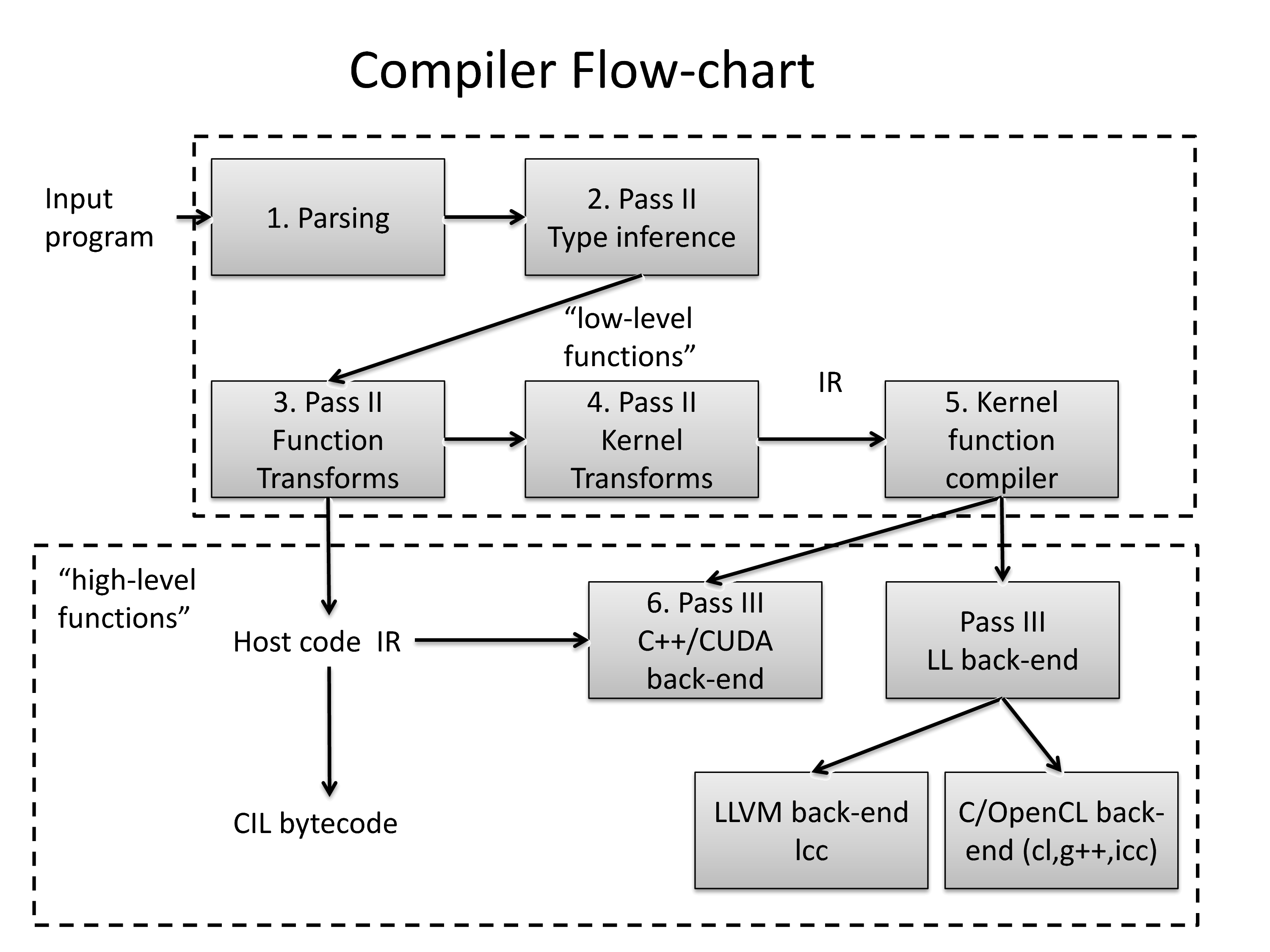
The function and kernel transforms will be discussed in the following sections in more detail.
17.1 Function Transforms
The Quasar compiler supports several function transforms:
\tightlist
- Automatic loop parallelization/serialization: performs automatic parallelization or serialization of loops within a function. Both for-loops and while-loops can be handled.
- Automatic kernel generator: vectorizes matrix expressions and generates corresponding kernel functions.
- Function optimization: performs ‘generic’ function optimization steps, such as constant folding, index packing, loop unrolling and elimination of dead branches etc.
- Function data transfer optimizer: annotates arguments of functions in such a way that the run-time system has less work (e.g., less memory copies required). Typically, when a matrix is only read from, its dirty bit does not need to be changed (possibly reducing the required number of data transfers)
- Boundary accessor transform: adds boundary accessor functions (see above) for newly generated array indexers
- Lambda to regular function converter: converts lambda expressions to regular functions that can be further optimized using the kernel transform pipeline, allowing the lambda expressions to be treated and optimized in the same way as regular functions
- High level inference: performs high-level inference of certain operations.
- Automatic function instantiation: automatic instantiation/specialization of functions
- Automatic kernel specialization: automatically specializes kernel functions
- Function inlining transform: inlines function calls annotated with the $inline meta-function (see Section 8.6↑), uses heuristics to inline functions automatically depending on the optimization level
- Dynamic memory handler: manages and checks the use of dynamic kernel memory inside kernel functions.
- Generic function predicator: detects functions (typically device/kernel functions) that are generic and that need to be specialized
- Imperfect loop optimization: converts certain types of imperfect loops to perfect loops that can be parallelized using the automatic loop parallelizer.
- Device function parallelizable test: checks whether a device function can be executed in parallel (useful for automatic loop parallelization)
- Shared memoy promotion: modifies kernel functions to use shared memory as a cache, typically due to the use of shared memory designators (see Section 9.2↑).
- Modular optimization framework: a group of interprocedural optimizations, such as schedule reordering optimizations, memory resource optimization and kernel fusion (see Subsection 17.1.6↓).
- Kernel post-processor: invoking the kernel transform pipelines and generating target-specific code.
Some of the function transforms are highlighted below.
17.1.1 Automatic For-Loop Parallelizer (ALP)
The ALP automatically parallelizes multi-dimensional loops (of arbitrary dimension) in the code, generating a kernel function and corresponding parallel_do call. In case of dependencies between the iterations of the for-loop, it is also possible that a serial_do call is generated. In that case, the loop will be executed serially on the CPU.
The ALP attempts to parallelize starting with the outside loops. The ALP program automatically recognizes one, two or higher dimenional for-loops, and also maximizes the dimensionality of the loops subject to parallelization.
During parallelization of for-loops, several compiler errors may be generated. These compiler errors can be classified in four categories: 1) errors related to dependency problems, 2) errors related to features that are currently not supported by the ALP, 3) issues related to the use of dynamic kernel memory and 4) attempts to call host functions from the loop. The errors are now discussed in more detail:
-
Dependency problems:\begin_inset Separator latexpar\end_insetIn case of dependency problems, the loop cannot be parallelized but will rather be serialized. In some cases, it is useful to modify the algorithm to get rid of the dependency.\tightlist
- Parallelization not possible: dependency on iterator variable!
It is also possible to force a loop to be parallelized irrespective of the warnings, using{!parallel for}. Note that this is at the responsibility of the user - the result may be incorrect if there are data races. -
Unsupported features:\begin_inset Separator latexpar\end_insetSome features are currently unsupported by the loop parallelizer. For example, the types of the variables must be determined statically.\tightlist
- Operations involving strings can currently not be parallelized/serialized.
- Operations involving objects can currently not be parallelized/serialized.
- Construction of cell arrays can not be parallelized/serialized.
- Statement can not be parallelized/serialized. Consider placing this outside the loop.
- Cannot use reserved variable name in this context.
- Parallelization/serialization not possible because the variable is polymorphic (not a unique type).
- Inner loop break detected. Loop cannot be parallelized/serialized.
- continue detected. Loop cannot be parallelized/serialized.
- Parallelization not possible because variable is not locally defined.
-
Kernel dynamic memory:\begin_inset Separator latexpar\end_insetOther parallelization operations result in dynamic memory use inside the kernel (which may degrade the performance on, e.g., a GPU). In particular, without dynamic kernel memory (see Section 8.3↑), matrix expressions such as A[:,2], B[3,4,:] can not be parallelized. This is because the size of the result is unknown to the compiler. When the result is a small vector (of length <= 32), the problem can be solved using the sequence syntax, with constant lower and upper bounds. For example: A[0..4,2], B[3,4,0..2].\tightlist
- Operator : can not be parallelized. Consider using [a..b] instead!
- Parallelization of the function requires kernel dynamic memory to be enabled!
- Operator requires dynamic kernel memory.
- Parallelization of the operator not possible: need to know the size of the result of type!
-
Calling host functions:\begin_inset Separator latexpar\end_insetHost functions cannot be called from a device/kernel function. Consequently, when a host function is directly called from a loop (and the host function cannot be inlined), the parallelization fails.\tightlist
- Function call can not be parallelized! Check if the function is declared with the __device__ modifier!
- Method is not a device function and can therefore not be parallelized/serialized!
- Parallelization/serialization not possible because the specified function is not a device or kernel function!
17.1.2 Automatic Kernel Generator
The automatic kernel generator extracts expression patterns that are used once, or multiple times throughout the code. For example:
function Z = f(A:mat,X:mat,Y:mat)
Z = A.*X+Y+4
endfunction
Z = A.*X+Y+4
endfunction
In this case, the expression A.*X*Y+T will be extracted and converted to a kernel function that can be evaluated with one single parallel_do function (instead of multiple kernels being called by the run-time). The generated kernel function will be:
function Z = opt1(A:mat,X:mat,Y:mat,T:scalar)
function [] = __kernel__ kernel(Z:mat,A:mat,X:mat,Y:mat,T:scalar,pos:ivec2)
Z[pos]=A[pos].*X[pos]+Y[pos]+T
endfunction
Z = uninit(size(A))
parallel_do(sizeof(Z),Z,A,X,Y,T,kernel)
endfunction
function [] = __kernel__ kernel(Z:mat,A:mat,X:mat,Y:mat,T:scalar,pos:ivec2)
Z[pos]=A[pos].*X[pos]+Y[pos]+T
endfunction
Z = uninit(size(A))
parallel_do(sizeof(Z),Z,A,X,Y,T,kernel)
endfunction
Additionally, a reduction is generated internally, allowing the reduction pattern to be reused for later optimizations:
reduction (A:mat,X:mat,Y:mat,T:scalar)->A.*X+Y+T = opt1(A,X,Y,T)
The code is then transformed into:
function Z = f(A:mat,X:mat,Y:mat)
Z = opt1(A,X,Y,4)
endfunction
Z = opt1(A,X,Y,4)
endfunction
Another purpose of the automatic kernel generator: the back-ends typically do not know how to handle high-level expressions such as (A:mat)+(B:mat), therefore this transform converts the operations to low-level calls that can be handled by the back-end. This may lead to nested kernel function calls, utilizing CUDA dynamic parallelism or OpenMP nested parallelism (see Section 4.4↑).
The automatic kernel generator is in a certain sense similar to the automatic loop parallelizer, with the main difference that the kernel generator starts from expressions involving matrices (but no indices) while the automatic loop parallelizer starts from loops involving matrices with indices (hence scalar values).
The automatic kernel generator also supports certain aggregation functions, such as sum, prod, max, min. When such a function is used, for example in expressions as sum(A.*B+C) the compiler will generate a parallel reduction algorithm to calculate the final result.
17.1.3 Automatic Function Instantiation
The automatic function instantiation step checks for certain conditions in which a (generic) function can be specialized:
- The function to be called is generic and requires specialization (e.g., because of a contained kernel function with generic arguments).
-
Some of the arguments of the function are generic device functions. In this case, a type deduction is performed for obtaining the generic parameters. For example, consider calling the following function:\begin_inset Separator latexpar\end_insetfunction y = apply[T](x : T, y : T, fn : [__device__ (T,T)->T])
y = fn(x,y)
endfunction
print apply(1,2,(__device__(x,y)->x+y))Here, the type deduction will find that T==int, so that the function fn ha type [__device__ (int,int)->int]. Correspondingly, the function apply can be specialized.
17.1.4 High Level Inference
The high-level inference transform infers high-level information from Quasar programs. High-level here refers to information on high-level data structure level (like vector/matrix level). The information can then be used in several later optimization stages.
Consider the following function:
function [output:cube] = overlay_labels(image:cube, nlabels:mat)
output = zeros(size(image))
function [] = __kernel__ draw_outlines(nlabelsk:mat’clamped,pos)
if nlabelsk[pos] == nlabelsk[pos+[0,-1]] && nlabelsk[pos] == nlabelsk[pos+[-1,0]]
%interior pixel
else
%edge pixel
output[pos[0],pos[1],0] = 1
output[pos[0],pos[1],1] = 1
output[pos[0],pos[1],2] = 1
endif
endfunction
parallel_do(size(input,0..1), nlabels, draw_outlines)
endfunction
The program contains some logic for converting a label image (where every segment has a constant value) into an image where the segment boundaries are all assigned the value 1.
Perhaps without knowing so, the programmer actually specifies a lot of extra information that the compiler can exploit. A first approach is type inference, which allows the compiler to generate code with “optimal” data types that can be mapped onto x86/64/GPU instructions.
However, there is actually a lot more high-level information available. For example, after the assignment output = zeros(size(image)), we know that size(output) == size(image). Combined with the parallel_do construct, we can determine that the boundary checks for output are actually unnecessary!
In fact, every statement has a number of pre-constraints, and after processing the statement, some post-constraints holds. For example, for the transpose function:
y = transpose(x)
% pre: ndims(x) <= 2
% post: size(y) = size(x,[1,0])
% pre: ndims(x) <= 2
% post: size(y) = size(x,[1,0])
For the matrix multiplication:
y = A * x
% pre: ndims(A) <= 2 && ndims(x) <= 2
% post: size(y) = [size(A,0), size(x,1)]
% pre: ndims(A) <= 2 && ndims(x) <= 2
% post: size(y) = [size(A,0), size(x,1)]
The constraints do not only help the compiler to find out mistakes (such as incompatible matrix dimensions), but can also be used for controlling the later optimization stages. For example:
for m=0..size(z,0)-1
for n=0..size(z,1)-1
z[m,n] = x[m,n] + y[m,n]
endfor
endfor
for n=0..size(z,1)-1
z[m,n] = x[m,n] + y[m,n]
endfor
endfor
If it is known that size(z)==size(x) && size(z) == size(y), then not only the boundary checks can be omitted, but also the loop can be flattened to a one dimensional loop, resulting in performance benefits on both CPU and GPU.
17.1.5 Function inlining
Functions can be inlined by annotating the function itself (C style inlining) or by annotating the function call with the $inline meta function (Section 8.6↑). Marking a function to be inlined can be done using {!auto_inline}:
function [x,y] = __device__ sincos(theta)
{!auto_inline}
[x,y] = [sin(theta),cos(theta)]
endfunction
{!auto_inline}
[x,y] = [sin(theta),cos(theta)]
endfunction
Alternative, the function can be inlined on a case by case basis (using $inline):
[a,b] = $inline(sincos)(0.3)In this example, the compile-time expansion will even lead to the result being calculated at compile-time.
The Quasar compiler also uses its own heuristics to automatically inline functions. By default lambda expressions are inlined differently than functions (for lambda functions {!auto_inline} can not be used). The lambda expression inlining mode depends on the COMPILER_LAMBDAEXPRESSION_INLINING setting (see Section 17.3↓), which has the following values:
- Never: never inline any lambda expressions
- Always: automatically inline every lambda expression
- OnlySuitable (default): only inlines “simple” lambda expressions that do not have closures.
Note that the back-end compilers may aggressively inline device functions, even without inlining being specified on the Quasar language level.
17.1.6 Kernel fusion
Nowadays, it is not uncommon that a convolution operation on a Full HD color image takes around 10 microseconds. However, with execution times so low, for many GPU libraries this has the consequence that the bottleneck moves back from the GPU to the CPU: the CPU must ensure that the GPU is busy at all times. This turns out to be quite a challenge on its own: when invoking a kernel function, there is often a comined runtime and driver overhead in the order of 5-10 microseconds. That means that all launched kernel functions must provide sufficient workload. Because just a filtering operation on a Full HD image is already in the 5-10 microsecond range of execution time, many smaller parallel operations (e.g., operations with data dimensions< 512⋅1024) are often not suited anymore for the GPU, unless the computation is sufficiently complex. In the new features of CUDA 10 it is mentioned:
“The overhead of a kernel launch can be a significant fraction of the overall end-to-end execution time.”
CUDA 10 introduces a graph API, which allows kernel launches to be prerecorded in order to be played back many times later. This technique reduces CPU kernel launch cost, often leading to significant performance improvements. We notice however that CUDA graphs are a runtime technique; its compile-time equivalent is kernel fusion. In kernel fusion, several subsequent kernel launches are fused into one big kernel launch (called a megakernel). In older versions of CUDA, dependent kernels could not easily be fused, because every kernel execution imposes an implicit grid synchronization at the end of execution. This grid synchronization could only be avoided by using CUDA streams which allows independent kernels to be processed concurrently. More recently, grid barriers (which synchronizes "all threads" in the grid of a kernel function) have become available, either via cooperative groups (in CUDA 9) or via emulation techniques. These grid barriers open the way to kernel fusion of dependent kernels.
Obviously, any synchronization point such as a grid barrier involves a certain overhead, a time that GPU threads spend waiting for other threads to complete. The total overhead can be minimized by minimizing the number of synchronization points. On the other hand, grid barriers are entirely avoided when there are no dependencies between the kernels. This automatically means that reordering of kernel launches is an essential step of the automatic kernel fusion procedure.
The application of compile-time kernel fusion also has several other performance related benefits: when multiple kernels become one kernel often temporary data stored in global memory can be entirely moved to the GPU registers. Since accessing GPU registers is significantly faster than reading from/writing to global memory, the execution performance of kernels can be vastly improved. In addition, the compiler can reuse memory resources and eliminate memory allocations, essentially leading a static allocation scheme, in which all temporary buffers are preallocated, prior to launching the megakernel.
The kernel fusion also has a number of complicating factors:
- It is neccessary to determine at compile-time that arrays (vectors, matrices, ...) have the same size. Luckily, Quasar’s high level inference engine allows to achieve this.
- Kernels are often launched with different data (i.e., grid and block) sizes, while launching a megakernel requires one size to be passed. In Quasar, this is achieved by performing automatic kernel tiling.
- Kernels often operate on data of different dimensionalities (vector, matrix, ...). In Quasar, this is solved by performing a kernel flattening transform in combination with a grid-strided loop.
The remedies for different data dimensions each involve a separate overhead, usually in the form of more registers used by the megakernel. This may lead to register-limited kernel launches, in which some GPU multiprocessors are underutilized because of insufficient register memory. Therefore, Quasar includes a dynamic programming based optimization algorithm that takes all these factors into account.
In short, kernel fusion in Quasar is achieved by placing:
inside the parent function of the kernel functions. Important to realize is that all functions called by this parent function are inlined, so that if the callees launch kernel functions on their own, these kernel fusions can also be fused into the mega kernel. The compiler therefore sees a sequence of kernel launches and has to determine 1) a suitable order to launch the kernels and 2) whether the kernels are suited to perform kernel fusion.
{!kernel_fusion strategy="smart"}
When performing kernel fusion, a strategy needs to be passed, which controls the cost function used by the optimization algorithm:
| Kernel fusion strategy | Purpose |
| smart | Let the Quasar compiler decide what is the best strategy |
| noreordering | Performs kernel fusion, without reordering the kernel launches |
| minsyncgrid | Minimizes the number of required grid synchronization barriers |
| minworkingmemory | Minimizes the total amount of (global) memory required for executing the fused kernel |
| manual | Kernel fusion barriers placed in the code determine which kernels are fused |
Kernel fusion barriers {!kernel_fusion barrier} may be added to prevent kernels from being fused. In this case, M kernels are fused into N kernels with 1 < N ≤ M.
Under some circumstances (which also depend on the kernel fusion strategy), the compiler may waive fusion of certain kernels. The reasons can be inspected in the kernel fusion code transform log, which is accessible through the code workbench window in Redshift.
17.2 Kernel transforms
Various kernel transforms are available, that are specialized to parallel or serial loops:
- Closure variable promotion pass: promotes closure variables of kernel functions to fully fledges function parameters, at least whenever possible/advantageous.
- Auto vectorization: automatically vectorizes code, making it more suitable for execution on SIMD processors.
- Branch divergence reducer: converts conditional computations into equivalent branch-free expressions, with the goal to reduce branch divergence on a GPU
- Kernel flattening: reduces the dimensionality of loops whenever possible. Loops of lower dimensionality are often more efficient due to the smaller number of registers being used by the resulting kernel function.
- Kernel data access scout: performs some scanning and annotating operations necessary for later optimization steps.
- Kernel dimension interchange: changes the order of the loops in a multi-dimensional for loop
- Memory coalescing transform: automatically detects lack of memory coalescing and suggests an appropriate dimension interchange to improve memory coalescing.
- Demultiplexer: splits up the compilation streams, allowing target-dependent code to be generated
- Kernel tiling: tiles the iterations of a loop; useful for loop unrolling and vectorization. Additional benefits on CUDA architectures.
- Parallel reduction transform: converts loops with +=, *= etc. accumulation patterns to the parallel reduction algorithm.
- Parallel dimension reduction transform: same as the parallel reduction transform, but also works for aggregation along one dimension and for parallel prefix sum patterns.
- Local windowing transform: Caches global memory into shared memory, in order to reduce memory access times. Mainly useful for targetting GPUs
- CPU skeleton generation: Generates skeleton code for the CPU so that the kernel function can run efficiently on x86/x64 and ARM architectures. The pass may take information generated during previous passes into account (e.g. to enable vectorization of instructions)
- Boundary accessor transform: adds boundary accessor functions (see above) for newly generated array indexers
- Shared memory caching transform: caches some of the input/output matrices in shared memory. Useful for, e.g., histogram calculation.
- Remove singleton matrix dimensions: replaces matrices or cubes with singular dimensions by lower-dimensional versions of those. This allows the indexing to be performed more efficiently (eliminating multiplication operations with dimension 1).
- Target-specific optimization transform: performs some user-defined target-specific optimizations (usually based on the $target() meta function).
- Avanced post optimization: scans for several suboptimal patterns generated by other kernel transforms and replaces these patterns by more efficient versions.
- SIMD processing: automatically vectorizes code, depending on the default vector length for the target architecture
Some of the transforms are described in more detail below.
17.2.1 Parallel Reduction Transform
The parallel reduction transform (PRT) is specifically useful for GPU target platforms (CUDA/OpenCL), exploiting both the thread synchronization and shared memory capabilities of the GPU. The PRT detects a variety of accumulation patterns in output variables, such as result += 1.0. The accumulation operator is always an atomic operator (e.g., atomic add +=, atomic multiply *=, atomic minimum __=, atomic maximum ^^=).
The following is an example of an accumulation patterns where the PRT can be applied:
The following is an example of an accumulation patterns where the PRT can be applied:
y = y2 = 0.
for m=0..size(img,0)-1
for n=0..size(img,1)-1
y += img[m,n]
y2 += img[m,n].^2
endfor
endfor
for m=0..size(img,0)-1
for n=0..size(img,1)-1
y += img[m,n]
y2 += img[m,n].^2
endfor
endfor
This loop can be executed in parallel using atomic operations, however this may cause a poor performance. The parallel reduction transform converts the above pattern to: [N] [N] Actual implementation details may vary for different versions of Quasar.
function [y:scalar,y2:scalar] = __kernel__ kernel(img:vec’const,$datadims:int,blkpos:int,blkdim:int)
$bins=shared(blkdim,2)
$accum0=$accum1=0
$m=blkpos
$bins=shared(blkdim,2)
$accum0=$accum1=0
$m=blkpos
while $m<$datadims
$accum1+=$getsafe(img,$m)
$accum0+=($getsafe(img,$m).^2)
$m+=blkdim
endwhile
$accum1+=$getsafe(img,$m)
$accum0+=($getsafe(img,$m).^2)
$m+=blkdim
endwhile
$bins[blkpos,0]=$accum0
$bins[blkpos,1]=$accum1
syncthreads
$bit=1
$bins[blkpos,1]=$accum1
syncthreads
$bit=1
while $bit<blkdim
if mod(blkpos,(2*$bit))==0
$bins[blkpos,(0..1)]=($bins[blkpos,(0..1)]+$getsafe($bins,(blkpos+$bit),(0..1)))
endif
if mod(blkpos,(2*$bit))==0
$bins[blkpos,(0..1)]=($bins[blkpos,(0..1)]+$getsafe($bins,(blkpos+$bit),(0..1)))
endif
syncthreads
$bit*=2
endwhile
$bit*=2
endwhile
if sum(blkpos)==0
y2+=$bins[0,0]
y+=$bins[0,1]
endif
endfunction
y2+=$bins[0,0]
y+=$bins[0,1]
endif
endfunction
The parallel reduction transform relieves the user from writing complicated parallel reduction algorithms. Accumulator variables can have scalar, cscalar, int, vecX, cvecX and ivecX datatypes. The transform calculates the required amount of shared memory and ensures that the kernel is not performance limited due to shared memory pressure. For CUDA 9 (or newer) backends, the parallel reduction transform switches to a warp-shuffling based algorithm when too many accumulator variables are present. It is even possible to specify per accumulator variable which parallel reduction algorithm needs to be used:
y = y2 = 0.
for m=0..size(img,0)-1
for n=0..size(img,1)-1
{!kernel_accumulator name=y; algorithm="warpshuffle"}
{!kernel_accumulator name=y2; algorithm="sharedmemory"}
y += img[m,n]
y2 += img[m,n].^2
endfor
endfor
Table 17.1↓ lists available parallel reduction algorithms. atomicop leads possibly to the least efficient algorithm but is available as alternative (e.g., for platforms on which warp shuffling is not supported).
for m=0..size(img,0)-1
for n=0..size(img,1)-1
{!kernel_accumulator name=y; algorithm="warpshuffle"}
{!kernel_accumulator name=y2; algorithm="sharedmemory"}
y += img[m,n]
y2 += img[m,n].^2
endfor
endfor
Table 17.1 Available parallel reduction algorithms
| Algorithm | Purpose |
| default | Lets the compiler choose the most suitable parallel reduction algorithm |
| sharedmemory | Performs the parallel reduction in shared memory |
| warpshuffle | Performs the parallel reduction using warp shuffling operations (CUDA 9 or higher) |
| atomicop | Uses a grid-strided loop in combination with an atomic operation |
17.2.2 Local Windowing Transform
The local windowing transform is designed to improve local windowing operations (also known as stencil operations), such as in convolutions, morphological operations. The transform is again useful for code that has to run on the GPU. Currently, the transform needs to be enabled with {!kernel_transform enable="localwindow"}.
function [] = __kernel__ joint_box_filter_hor(g : mat’mirror, x : mat’mirror, tmp_g : mat’unchecked, tmp_x : mat’unchecked, tmp_gx : mat’unchecked, tmp_gg : mat’unchecked, r : int, pos : vec2)
{!kernel_transform enable="localwindow"}
s_g = 0.
s_x = 0.
s_gx = 0.
s_gg = 0.
for i=-r..r
t_g = g[pos + [0,i]]
t_x = x[pos + [0,i]]
s_g = s_g + t_g
s_x = s_x + t_x
s_gx = s_gx + t_g*t_x
s_gg = s_gg + t_g*t_g
endfor
tmp_g[pos] = s_g
tmp_x[pos] = s_x
tmp_gx[pos] = s_gx
tmp_gg[pos] = s_gg
endfunction
{!kernel_transform enable="localwindow"}
s_g = 0.
s_x = 0.
s_gx = 0.
s_gg = 0.
for i=-r..r
t_g = g[pos + [0,i]]
t_x = x[pos + [0,i]]
s_g = s_g + t_g
s_x = s_x + t_x
s_gx = s_gx + t_g*t_x
s_gg = s_gg + t_g*t_g
endfor
tmp_g[pos] = s_g
tmp_x[pos] = s_x
tmp_gx[pos] = s_gx
tmp_gg[pos] = s_gg
endfunction
This is translated into:
function [] = __kernel__ joint_box_filter_hor(g:mat’const’mirror,x:mat’const’mirror,tmp_g:mat’unchecked,tmp_x:mat’unchecked,tmp_gx:mat’unchecked,tmp_gg:mat’unchecked,r:int,pos:ivec2,blkpos:ivec2,blkdim:ivec2)
{!kernel name="joint_box_filter_hor"; target="gpu"}
sh$x=shared((blkdim+[1,((r+r)+1)]))
sh$x[blkpos]=x[(pos+[0,-(r)])]
{!kernel name="joint_box_filter_hor"; target="gpu"}
sh$x=shared((blkdim+[1,((r+r)+1)]))
sh$x[blkpos]=x[(pos+[0,-(r)])]
if (blkpos[1]<(r+r))
sh$x[(blkpos+[0,blkdim[1]])]=x[(pos+[0,-(r)]+[0,blkdim[1]])]
endif
sh$x[(blkpos+[0,blkdim[1]])]=x[(pos+[0,-(r)]+[0,blkdim[1]])]
endif
blkof$x=((blkpos-pos)-[0,-(r)])
sh$g=shared((blkdim+[1,((r+r)+1)]))
sh$g[blkpos]=g[(pos+[0,-(r)])]
sh$g=shared((blkdim+[1,((r+r)+1)]))
sh$g[blkpos]=g[(pos+[0,-(r)])]
if (blkpos[1]<(r+r))
sh$g[(blkpos+[0,blkdim[1]])]=g[(pos+[0,-(r)]+[0,blkdim[1]])]
endif
sh$g[(blkpos+[0,blkdim[1]])]=g[(pos+[0,-(r)]+[0,blkdim[1]])]
endif
blkof$g=((blkpos-pos)-[0,-(r)])
syncthreads
s_g=0.
s_x=0.
s_gx=0.
s_gg=0.
for i=-(r)..r
t_g=sh$g[(pos+[0,i]+blkof$g)]
t_x=sh$x[(pos+[0,i]+blkof$x)]
s_g=(s_g+t_g)
s_x=(s_x+t_x)
s_gx=(s_gx+(t_g*t_x))
s_gg=(s_gg+(t_g*t_g))
endfor
tmp_g[pos]=s_g
tmp_x[pos]=s_x
tmp_gx[pos]=s_gx
tmp_gg[pos]=s_gg
endfunction
syncthreads
s_g=0.
s_x=0.
s_gx=0.
s_gg=0.
for i=-(r)..r
t_g=sh$g[(pos+[0,i]+blkof$g)]
t_x=sh$x[(pos+[0,i]+blkof$x)]
s_g=(s_g+t_g)
s_x=(s_x+t_x)
s_gx=(s_gx+(t_g*t_x))
s_gg=(s_gg+(t_g*t_g))
endfor
tmp_g[pos]=s_g
tmp_x[pos]=s_x
tmp_gx[pos]=s_gx
tmp_gg[pos]=s_gg
endfunction
17.2.3 Kernel Tiling Transform
Kernel tiling is a kernel function code transformation that divides the data in blocks of a fixed size. There are three possible modes:
-
Global kernel tiling: the data is subdivided in blocks of, e.g., ‘32x32x1‘ or ‘32x16x1‘. All threads in the grid collaborate to first calculate the first block, then the second block, and so on. The loop that traverses all these blocks is placed inside the kernel function. Note that the blocks normally don’t corresponds to the GPU (CUDA) blocks. It is very common that a 1D block index traverses 2D or 3D blocks (also called grid-strided loop). Global kernel tiling has the following benefits:
- Threads are reused; the maximum number of GPU blocks can be reduced, saving thread initialization and destruction overhead
- Calculations independent of the block can be placed outside of the tiling loop
- Less dependency on the GPU block dimensions, resulting in more portable code
A disadvantages of global kernel tiling is that the resulting kernels are more complex and typically use more registers.Global kernel tiling can be activated by placing one of the following code attributes in the kernel function:{!kernel_tiling dims=[32,16,1]; mode="global"; target="gpu"}
{!kernel_tiling dims=auto; mode="global"; target="gpu"}The target (e.g., cpu, gpu) specifies for which platform the kernel tiling will be performed. It is possible to enable tiling for one platform but not for the other. By combining multiple code attributes it is also possible to specify different block sizes for different platforms. In case of automatic tiling dimensions, the runtime will search for suitable block dimensions that optimize the occupancy.For certain kernels (e.g., involving parallel reduction, shared memory accumulation, ...), global kernel tiling is performed automatically. Kernels that use grid-level synchronization primitives (without TCC driver mode cooperative grouping) are also automatically tiled globally. This is also required in order for kernel fusion (see Subsection 17.1.6↑) to work correctly. -
Local kernel tiling: here, each thread performs the work of N consecutive work elements. Instead of having 1024 threads process a block of size 32 × 32, we have 256 threads processing the same block. Each thread then processes data in a single instruction multiple data (SIMD) fashion. Moreover, the resulting instructions can be even mapped onto SIMD instructions (e.g., CUDA SIMD/SSE/AVX/ARM Neon, see also Chapter 12↑), if the hardware supports them. In the following example, a simple box filter is applied to a matrix with element type uint8.function [] = __kernel__ conv(im8 : mat[uint8], im_out : mat[uint8], K : int, pos : ivec(2))Local kernel tiling can be activated by placing the following code attribute in the kernel function: {!kernel_tiling dims=[1,1,4]; mode="local"; target="gpu"}In case purely SIMD processing is intended, it is better to use the following code attribute (see below):{!kernel_transform enable="simdprocessing"}Advantages of local kernel tiling:
[m,n] = pos
r2 = vec[int](4)
for x=0..K-1
r2 += im8[m,n+x+(0..3)]
endfor
im_out[m,n+(0..3)] = int(r2/(2*K))
endfunction- Less threads, so less thread initialization and destruction overhead
- mapping onto SIMD possible (when the block dimensions are chosen according to the GPU platform).
- For some operations, recomputation of values can be avoided
Disadvantages:- The resulting kernels use more registers, which may negatively impact the performance in some cases (e.g. register limited kernels)
- Not all operations may be accelerated by hardware SIMD operations (for example, division operations).
- The compiler needs to ensure that the data dimensions are a multiple of the block size. If this is not the case, extra "cool down" code is added.
-
Hybrid tiling: combines the advantages of global and local kernel tiling. To activate hybrid tiling, code attributes for both local and global tiling can be placed inside the kernel function: {!kernel_tiling dims=auto; mode="global"; target="gpu"}Hybrid kernel tiling usually occurs as a result of several compiler optimizations.
{!kernel_tiling dims=[1,1,4]; mode="local"; target="gpu"}
Example
Consider the following convolution example:
for m=0..size(im,0)-1
for n=0..size(im,1)-1
{! kernel_tiling dims=[1,32]; mode="local"; target="cpu"}
r = 0.0
for x=-K..K
r += im[m,n+x]
endfor
im_out[m,n] = r/(2*K+1)
endfor
endfor
for n=0..size(im,1)-1
{! kernel_tiling dims=[1,32]; mode="local"; target="cpu"}
r = 0.0
for x=-K..K
r += im[m,n+x]
endfor
im_out[m,n] = r/(2*K+1)
endfor
endfor
This is translated into:
function [] = __kernel__ opt___kernel$2(K:int,im:mat’const,im_out:mat’unchecked,$datadim:ivec2)
$nMax=$cpu_gridDim().*$cpu_blockDim()
{!parallel for; private=r; private=x}
for $p1=0..$nMax[1]-1
for $p2=0..$nMax[0]-1
pos=[$p1,$p2]
r=zeros(32)
for x=-K..K
r+=im[pos[0],32.*pos[1]+(0..31)+x)]
endfor
im_out[pos[0],32.*pos[1]+(0..31)]=r./((2.*K)+1)
endfor
endfor
endfunction
$nMax=$cpu_gridDim().*$cpu_blockDim()
{!parallel for; private=r; private=x}
for $p1=0..$nMax[1]-1
for $p2=0..$nMax[0]-1
pos=[$p1,$p2]
r=zeros(32)
for x=-K..K
r+=im[pos[0],32.*pos[1]+(0..31)+x)]
endfor
im_out[pos[0],32.*pos[1]+(0..31)]=r./((2.*K)+1)
endfor
endfor
endfunction
The operations im[pos[0],32.*pos[1]+(0..31)] are translated to vector operations.
17.2.4 Kernel Boundary Checks
The Kernel Boundary Check transform detects index-out-of-bounds at compile-time, given the available information (i.e., through the truth-value system).
In certain cases, the transform can detect that the index will always be inside the bounds. In this case, the kernel argument type can have the modifier ’unchecked (omitting the boundary checks).
For example, the code fragment:
assert(size(A) == size(B))
parallel_do(size(A),A,B,
__kernel__ (y : mat,x : mat,pos : vec2) -> y[pos] += 4.0 * x[pos])
parallel_do(size(A),A,B,
__kernel__ (y : mat,x : mat,pos : vec2) -> y[pos] += 4.0 * x[pos])
Can be translated into:
parallel_do(size(A),A,B,
__kernel__ (y : mat’unchecked,x : mat’unchecked,pos : vec2) -> y[pos] += 4.0 * x[pos])
__kernel__ (y : mat’unchecked,x : mat’unchecked,pos : vec2) -> y[pos] += 4.0 * x[pos])
17.2.5 Target-specific programming and manually invoking the runtime scheduler
By default, the Quasar compiler takes a single kernel function as input and specializes the kernel function to multiple devices (e.g., CPU, GPU). In some circumstances, it may be desirable to manually write implementations for certain performance-critical functions for several targets. This can be achieved by either 1) writing multiple kernel functions and by indicating the compilation target within each kernel function (this section) or 2) using the $target() meta-function (Subsection 17.2.6↓). The compilation target of a kernel function can be specified using:
{!kernel name="gpu_kernel"; target="gpu"}Here, gpu_kernel indicates the name of the kernel function (which should correspond to the function definition). Several target identifiers are listed in Table 17.2↓. Depending on the compilation mode, it may happen that no code is generated for a given kernel function (for example, a GPU kernel when compiling in CPU mode). To decide which kernel function implementation is used, the schedule function needs to be used which has mostly the same arguments as the parallel_do function, with exception of the last parameter which takes a cell vector of the kernel function implementation. The schedule function returns a zero-based index of the selected kernel function passed via the cell vector.
Because schedule on its own does not trigger parallel_do, the schedule function is best used within a match control structure. Within the control structure, also additional launching code could be placed (like calculation of the optimal launch configuration, e.g., using the max_block_size, opt_block_size and opt_block_cnt functions). An example is given below for a sum algorithm using the parallel reduction pattern. Actually, for illustrational purposes: this is the parallel reduction code that is generated for the map-reduce pattern from Section 8.4↑.
Table 17.2 Supported target platform identifiers
| Target platform identifier | Description |
| cpu | Generic CPU target |
| gpu | Generic GPU target |
| nvidia_cuda | NVidia CUDA target (NVidia GPUs supporting CUDA) |
| nvidia_opencl | NVidia OpenCL target |
| nvidia | All NVidia targets |
| amd_opencl | AMD OpenCL target |
| amd | All AMD targets |
| generic_opencl | All other OpenCL targets |
| opencl | All OpenCL targets |
function y = manual_map_sum(x : vec, map : [__device__ (scalar)->scalar])
% GPU implementation
function y = __kernel__ gpu_kernel(x : vec’unchecked, nblocks : int,
map : [__device__ (scalar) -> scalar], blkdim : int, blkpos : int)
{!kernel name="gpu_kernel"; target="gpu"}
bins = shared(blkdim)
% step 1 - parallel sum
val = 0.0
for n=0..nblocks-1
if blkpos + n * blkdim < numel(x)
val += map(x[blkpos + n * blkdim])
endif
endfor
bins[blkpos] = val
% step 2 - reduction
syncthreads
bit = 1
while bit<blkdim
index = 2*bit*blkpos
if index+bit<blkdim
t = bins[index] + bins[index+bit]
bins[index] = t
syncthreads
endif
bit *= 2
endwhile
if blkpos==0
y = bins[0]
endif
endfunction
% Implementation using OpenMP
function y = __kernel__ cpu_kernel(x : vec’unchecked,
map : [__device__ (scalar) -> scalar])
{!kernel name="cpu_kernel"; target="cpu"}
val = 0.0
% The following special directive activates OpenMP to perform
% a parallel reduction. {!parallel for} is indended to
% eliminate #pragma force_parallel in the long term; since
% it provides a means to specify special attributes.
{!parallel for; reduction={val,"+="}}
for n=0..numel(x)-1
val += map(x[n])
endfor
y = val
endfunction
% Manually call the scheduler with two implementations
% In each case, we need to do some additional work
match schedule(numel(x), x, map, {gpu_kernel, cpu_kernel}) with
| 0 ->
N = numel(x)
BLOCK_SIZE = prod(max_block_size(gpu_kernel, N))
nblocks = int((N + BLOCK_SIZE-1) / BLOCK_SIZE)
y = parallel_do([[1,BLOCK_SIZE],[1,BLOCK_SIZE]],x,nblocks,map,gpu_kernel)
| 1 ->
y = serial_do(1,x,map,cpu_kernel)
endmatch
endfunction
In this example, two kernel functions have been implemented: one for respectively the GPU and the CPU. The GPU implementation uses the parallel reduction algorithm based on shared GPU memory (see Section 9.7↑), while the CPU implementation relies on the OpenMP parallel reduction pragma. The scheduling function is then called to determine the best suitable target for this operation. Subsequently, when the scheduler selects the GPU, additional launch configuration code is executed and the resulting parameters are passed to the parallel_do function.
Note that the parameter lists of cpu_kernel and gpu_kernel do not need to be equal. For schedule, it suffices to pass the relevant parameters that affect the scheduling decision.
17.2.6 Compile-time specialization through the $target() meta function
Optionally, kernel functions can use the $target() meta function for the implementation of target-specific code, for example:
if $target("nvidia_cuda")
% We are compiling for CUDA targets
else
% All other targets
endif
% We are compiling for CUDA targets
else
% All other targets
endif
The $target function is evaluated at compile-time during a target-specific optimization step. The function returns 1 in case we are compiling for the specified target and 0 otherwise. For the possible values accepted by the $target function, see Table 17.2↑.
Such approach is similar to preprocessor tests often used in C or C++ code. To keep the code readibility high, the technique can best be used when the amount of target-specific code is reasonably small (for example at most a few lines of code), otherwise it is recommended to write multiple kernel implementations (seeSubsection 17.2.5↑).
17.3 Common compilation settings
Compilation settings can be configured in the config file Quasar.config.xml. This file is stored in %APPDATA%\..\Local\Quasar (windows) or ~/.config/Quasar (linux). A number of global settings are listed in Table 17.3↓. Some of the global settings can also be modified in the program, using the #pragma directive. The following pragmas are available:\begin_inset Separator latexpar\end_inset
| #pragma loop_parallelizer (on|off) | Turns off/activates the automatic loop parallelizer |
| #pragma show_reductions (on|off) | Enables/disables messages when reductions are applied. |
| #pragma expression_optimizer (on|off) | Enables/disables the expression optimizer. |
Table 17.3 Global compilation settings
| Setting | Value | Description |
| NVCC_PATH | path | Contains the path of the NVCC compiler shell script |
| (nvcc_script.bat or nvcc_script.sh) | ||
| CC_PATH | path | Contains the path of the native C/C++ compiler shell script |
| MODULE_DIR | directory | ’;’ separated list of directories to search for .q files (when using import) |
| INTERMEDIATE_DIR | directory | Intermediate directory to be used for compilation. |
| If none specified, the directory of the input file is used | ||
| COMPILER_PERFORM_REDUCTIONS | True/False | Enables reductions (reduction keyword) |
| COMPILER_REDUCTION_SAFETYLEVEL | off, safe, strict | Compiler safety setting for performing reductions |
| COMPILER_DISPLAY_REDUCTIONS | True/False | Displays the reductions that have been performed |
| COMPILER_DISPLAY_WARNINGS | True/False | Displays warnings during the compilation process |
| COMPILER_OUTPUT_OPTIMIZED_FILE | True/False | If true, the optimized .q file is written to disk (for verification) |
| COMPILER_EXPRESSION_OPTIMIZER | True/False | Enables automatic extraction and generation of |
| __kernel__ functions (see Subsection 17.1.2↑) | ||
| COMPILER_SHOW_MISSED_OPT_OPPORTUNITIES | True/False | Displays additional possibilities for optimization |
| COMPILER_AUTO_FORLOOP_PARALLELIZATION | True/False | Enables automatic parallelisation of for-loops (see Subsection 17.1.1↑) |
| COMPILER_SIMPLIFY_EXPRESSIONS | True/False | Simplifies branch expressions whenever possible |
| COMPILER_PERFORM_BOUNDSCHECKS | True/False | Performs boundary checking of unchecked variables (CPU engine only) |
| Useful for debugging mistakes in the use of the ’unchecked modifier. | ||
| COMPILER_PERFORM_NAN_INF_CHECKS | True/False | Generates code that automatically checks for NaN or Inf values |
| (experimental feature) | ||
| COMPILER_PERFORM_NAN_CHECKS | True/False | Generates code that automatically checks for NaN values |
| (experimental feature) | ||
| COMPILER_LAMBDAEXPRESSION_INLINING | Off,OnlySuitable,Always | Allows/disallows the inlining of lambda expressions |
| COMPILER_USEFUNCTIONPOINTERS | Always, | Controls the generation of kernel/device functions |
| SmartlyAvoid,Error | using function pointers | |
| COMPILER_OPTIMIZATIONLEVEL | Basic/Moderate/Full | Specifies the optimization level used for compiling Quasar programs |
| COMPILER_BACKEND_CPU | Default/... | CPU back-end compiler to be used |
| COMPILER_BACKEND_CUDA | NVidiaC, NVidiaRTC | CUDA back-end compiler to be used |
| COMPILER_BACKEND_OPENCL | OpenCLDriver | OpenCL back-end compiler to be used |
| COMPILER_BACKEND_GENERATE_HUMAN | True/False | Generates human readable code in the back-end stages |
| _READABLE_CODE | (at the cost of longer code) | |
| COMPILER_BACKEND_OUTPUTLINEINFO | True/False | Generate line number information in the binary files (.ptx). |
| Useful for debugging and profiling. | ||
| CUDA_BACKEND_TARGETARCHITECTURE | Default, sm_20, ... | NVIDIA Target compile architecture (corresponding to the |
| NVCC -arch option). See Section 17.4↓. | ||
| CUDA_BACKEND_FLUSHTOZERO | True/False | Flushes denormalized numbers to zero |
| CUDA_BACKEND_PRECISIONDIVISION | True/False | Use precision division function |
| CUDA_BACKEND_PRECISIONSQRT | True/False | Use precision square root function |
| CUDA_BACKEND_FASTMATH | True/False | Use faster mathemetical functions (at the cost of lower numerical accuracy) |
| CUDA_BACKEND_OPTIMIZATIONMODE | O0/O1/O2 | Sets the optimization level for compiling CUDA code |
| CUDA_BACKEND_DYNAMICPARALLELISM | True/False | Generates code that uses dynamic parallelism |
| (requires target architecture sm_35 or higher) | ||
| CUDA_BACKEND_COOPERATIVEGROUPS | True/False | Generates code that uses cooperative groups (requires CUDA 9.1 or higher) |
| CUDA_BACKEND_WARPSHUFFLING | True/False | Generates code that uses warp shuffling (requires CUDA 9.1 or higher) |
17.4 CUDA target architecture
The CUDA target architecture (compiler option CUDA_BACKEND_TARGETARCHITECTURE) specifies the name of the NIVDIA virtual GPU architecture to generate code for. Possible values are Default, sm_13, sm_20, sm_21, sm_30, sm_35, sm_37, sm_50, sm_52, sm_53, sm_50, sm_60, sm_61, sm_62, sm_70, sm_71, sm_72, sm_75. Table 17.4↓ gives an overview of common GPU architectures:
| Name | Architecture | CUDA versions | Example cards |
| Fermi | sm_20 | 3.2-8.0 | GeForce 400, 500, 600 |
| Kepler | sm_30 | 5.0+ | GeForce 700 |
| sm_35 | 5.0+ | Tesla K40 | |
| sm_37 | 5.0+ | Telsa K80 | |
| Maxwell | sm_50 | 6.0+ | Quadro M6000 |
| sm_52 | 6.0+ | Geforce 900, Titan X | |
| sm_53 | 6.0+ | Jetson TX1 | |
| Pascal | sm_60 | 8.0+ | Tesla P100 |
| sm_61 | 8.0+ | Geforce 1000, Titan Xp | |
| sm_62 | 8.0+ | Jetson TX2 | |
| Volta | sm_70 | 9.0+ | Tesla V100, TITAN V |
| Turing | sm_75 | 10.0+ | Geforce RTX 2080 Ti |
Table 17.4 Overview of CUDA target architectures
When the option ’Default’ is selected, the target architecture is automatically determined based on the installed graphics card. However, in some cases, it is useful to set a target architecture that differs from the default value:
- When generating CUDA code on a computer without NVIDIA GPU (for example, when building a library or binary to be deployed later on a system with NVIDIA GPU).
- When targetting older GPU cards.
GPU architectures are (generally) backward compatible. When compiling for sm_30, one can use the Geforce GTX 770, Titan X and even Titan Xp, but it is not possible to use older cards as the GeForce GTX 480. However, take into account that the sm_30 may not take advantage of features in newer generations of GPUs. Therefore, only when backward compatibility is an issue, it is useful to select a lower architecture than what your GPU supports.
On the other hand, some (very) old versions are not supported by the latest CUDA compiler. Therefore, it is recommended to use the option ’Default’, unless there is a specific reason to generate code for a lower GPU architecture.