Prev Chapter 17: The Quasar compiler/optimizer Up Main page

18 Development tools

Quasar comes with two main development tools: Redshift (the main IDE) and Spectroscope (a commandline debugger tool).

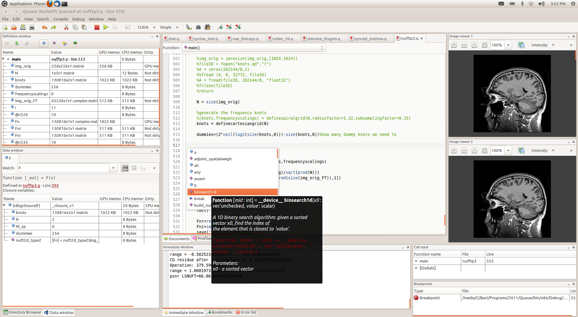
18.1 Redshift - integrated development environment

Redshift is the main IDE for Quasar. It is built on top of GTK and runs on Windows, Linux and MAC. Redshift has the following main features:

Multiple document editing with syntax highlighting and completion lists.
Built-in Quasar Spectroscope (see Section 18.2↓) for debugging and interactive programming
Call stack, variable definition, variable watch, breakpoints windows, ...
Incremental compilation, keeping binary modules (e.g., PTX) in memory: significantly decreases overall compilation time
Source code parsing, function browsing, comment parsing
Ability to break and continue running programs.
Integrated documentation system and help system
Integrated OpenGL functionality for fast visualization
2D and 3D image viewer
Advanced profiler tool with timeline view and special profiler code editor margin.
Interactive interpretation of Quasar commands
Data/image debug tooltips
Background compilation with source code error annotations
Optimization pipeline visualization

figure Figures/fig_Redshift_screenshot.png

Figure 18.1 Screenshot of the Redshift IDE for Quasar.

In the IDE, it is also possible to select the GPU devices on which the program needs to be executed in the main toolbar. Additionally, the precision mode (e.g., 32-bit floating point or 64-bit floating point) can be selected. The flame icon toggles concurrent kernel execution, a technique in which CUDA/OpenCL kernels are launched asynchronously; in many circumstances speeding up the execution.

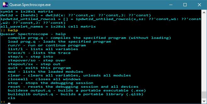
18.2 Spectroscope - command line debugger

Spectroscope is a command line debugger for Quasar. Its functionality is actually integrated in Redshift (Section 18.1↑), although in some circumstances it is still useful to use the debugging tools from a terminal in circumstances where a graphical environment is not available (e.g., over SSH on a remote server). Spectroscope provides an interactive environment where Quasar statements can be entered on interpreted on the fly. In addition, different commands are available:

compile [program.q]: compiles a specified program while checking for compilation errors
load [program.q]: compiles the specified program and loads the definitions (global variables and functions)
run: runs the loaded program
list: lists all variables within the current scope/context
trace: prints the current stack trace
step: performs a debugger step into a function
stepover: let’s the debugger step over the current statement
stepout: let’s the debugger step out of the current function
mod: lists all loaded Quasar modules
clear: clears all variables, unloads all loaded modules
path: prints the current module search directory
stop: terminates the current debugging session
reset: debugger hard reset - resets the debugging session and all devices
buildexe [program.q]: builds a portable executable file (.exe)
buildqlib [program.q]: builds a portable library (.qlib)
cls: clears the screen

figure Figures/fig_Spectroscope_screenshot.png

Figure 18.2 Screenshot of Quasar Spectroscope.

18.3 Redshift Profiler

To analyze the performance of Quasar programs, a profiler has been integrated in Redshift. The profiler uses the NVIDIA CUDA Profiling tools interface (CUPTI) to obtain accurate time measurements. Using the Redshift Profiler, it is not necessary to use the tools

nvprof

, NVIDIA Visual Profiler and NVIDIA nSight separately. The Redshift Profiler offers the following features:

Accurate kernel timing measurements with less profiling overhead
Integrated source correlation, to see instruction counts per code line
Detailed timeline view, linking kernel launches to the corresponding CPU activity
GPU events are linked with the corresponding CPU events (e.g.
```
parallel_do
```
or function call on the CPU).
Several detailed metrics are available for analyzing the performance of an individual kernel. Metrics include FLOPs/sec, integer operations/sec, branch efficiency, achieved occupancy, average number of instructions per second and many more.
Detailed GPU event view, to see individual operations performed on the GPU
Support for Multi-GPU profiling (e.g., peer to peer memory transfers)
Memory profiling: sub-tree view of memory allocations at any point in time

To take advantage of CUPTI, it is necessary to enable “Use NVIDIA CUDA profiling tools” in the program settings (done by default). Without this option set, the Quasar Profiler reverts to CUDA events (which is less accurate and degrades the performance during profiling).

In Windows,

cupti.dll

is bundled with the Quasar installation. In Linux, it may be necessary to adjust the

LD_LIBRARY_PATH

to include

libcupti.so

, depending on the installed version of CUDA. This can be done by modifying the

.bashrc

file (for example, for cuda 10.2):

export LD_LIBRARY_PATH=/usr/local/cuda-10.2/extras/CUPTI/lib64/:$LD_LIBRARY_PATH

The profiling menu in Redshift has been updated with the new features, as can be seen in the following screenshot:

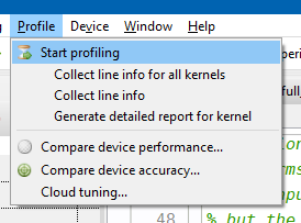
figure Figures/RedshiftProfiler-ProfilingMenu.png

The following features are available:

Start profiling: executes the program with the profiler attached. This will collect information about the CPU and GPU kernels, memory allocations, memory transfers\SpecialChar ldots
Collect line information for all kernels: executes all kernel functions in the current module with an execution tracer attached. This slows down the execution of the kernel functions. The results are displayed in the source code editor (see further).
Collect line information for a specific kernel: this is useful when you are optimizing one particular kernel
Generate detailed report for kernel: executes the program, collecting an extensive sets of metrics for the selected kernel function and generates a report (see below)
Compare device performance: useful to compare the execution performance of two devices (e.g. CUDA vs. OpenCL)
Compare device accuracy: checks the accuracy/correctness of the program by gathering statistics (e.g. minimum value, maximum value, average value of a matrix) during the execution of the program.
Cloud tuning: this feature is used to optimize the runtime scheduler and load balancer based on runtime measurements of kernels. The results (kernel execution times on CPU and GPU) are sent to the Gepura/Quasar server.

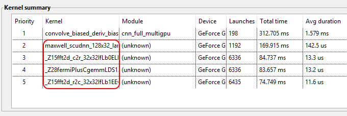
As a result of CUPTI, the profiler may now list kernel functions that are not visible to Quasar but that are launched by library calls (e.g., CuDNN, CuBLAS, CuFFT, \SpecialChar ldots). An example is given below:

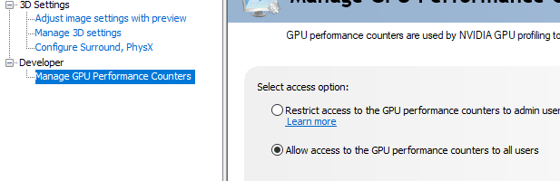
figure Figures/RedshiftProfiler-KernelSummary.png

18.3.1 Security settings

In CUDA 10.1 or newer, using cuPTI profiling requires an additional setting to be made. In Windows, open the NVIDIA control panel. Click on the desktop menu and enable the developer settings. Then, select “Manage GPU Performance Counters” and click on “Allow access to the GPU performance counters to all users” (see Figure 18.3↓). In Linux desktop systems, create a file /etc/modprobe.d with the following content:

options nvidia "NVreg_RestrictProfilingToAdminUsers=0"

where on some Ubuntu systems, nvidia may need to be replaced by nvidia-xxx where xxx is the version of the display driver (use lsmod | grep nvidia to find the number). In addition, it may be necessary to rebuild the ram FS:

update-initramfs -u

We recommend creating a backup of the initrd image first (see /boot directory).

For NVIDIA Jetson development boards, the modprobe approach is not available. The only way to get the cuPTI profiling to work is by executing Quasar or Redshift with admin rights, for example, using sudo.

For more information, see https://developer.nvidia.com/nvidia-development-tools-solutions-ERR_NVGPUCTRPERM-permission-issue-performance-counters#SolnAdminTag.

figure Figures/fig_ProfilingSecuritySettings.png

Figure 18.3 NVIDIA control panel: allow access to the GPU performance counters to all users

18.3.2 Peer to peer transfers

In multi-GPU configurations, the profiler now displays memory statistics for peer to peer memory copies (i.e., transfers between two GPUs). See the multi-GPU programming documentation for an explanation of the performance implications related to these peer to peer transfers.

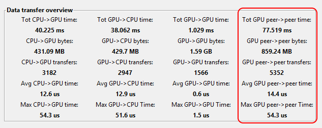
figure Figures/RedshiftProfiler-DataTransferOverview.png

When the profiler indicates memory transfer performance bottlenecks, it is possible to investigate every bottleneck individually, via the memory transfer summary.

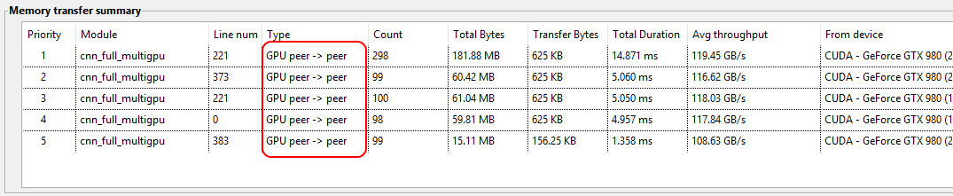
figure Figures/RedshiftProfiler-MemoryTransferOverview.png

Per line of code, the memory transfers are listed, including the following information:

Count: the number of transfers that were measured
Type: the type of transfer: CPU to GPU, GPU to CPU, GPU to GPU or peer to peer
Total Bytes: the total number of bytes for all memory transfers of this type
Transfer Bytes: the number of bytes transferred per transaction (Total bytes = Count * Transfer Bytes)
Total Duration: the total amount of time taken by the memory transfers of this type
Average throughput: the measured transfer speed.
From device: the device from which the transfer originates
To device: the device to which the transfer is done

In systems in which multiple GPUs are not connected to the same PCIe slot, the peer to peer copy between GPUs generally passes the CPU memory. Correspondingly, these peer-to-peer copies cause two transfers: 1) from the source GPU to the CPU host and 2) from the CPU host to the target GPU. In the memory transfer view, the peer to peer copies are listed as one operation, for clarity. In the timeline view however, such peer to peer copies are displayed as dual operations (in green in the screenshot below):

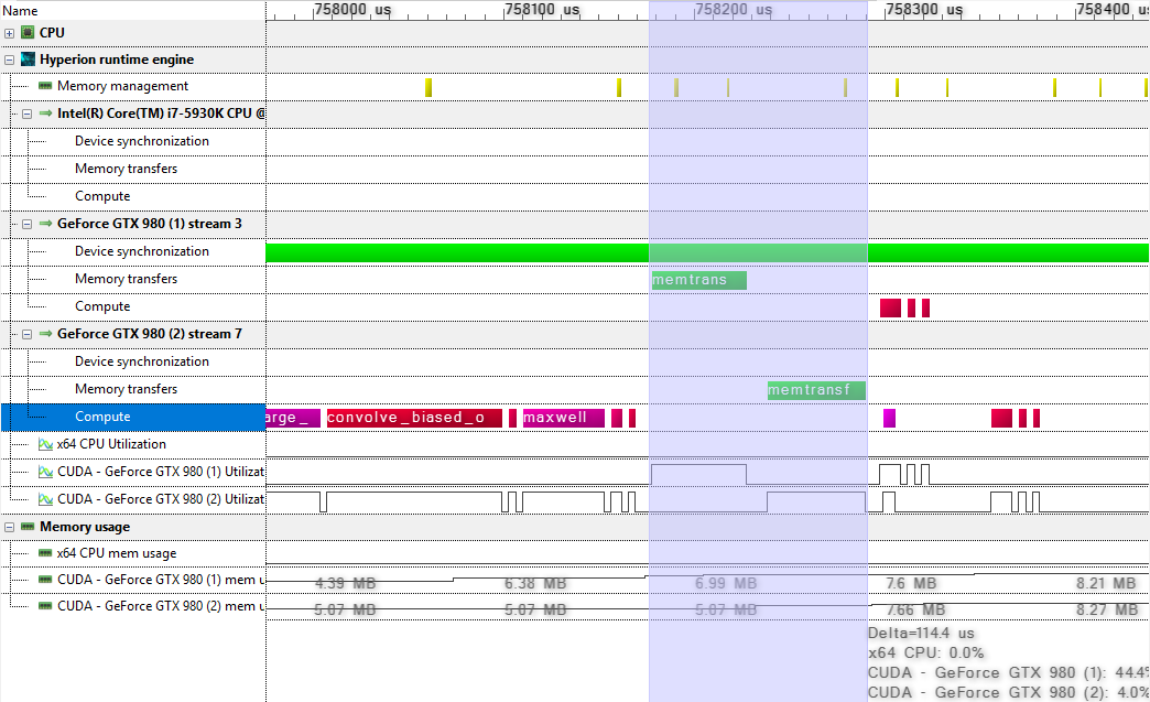
figure Figures/RedshiftProfiler-Peer2PeerCopyTimeline.png

In the screenshot, it can be seen that the peer to peer copy blocks all operations on both GPUs, which is degrades the runtime performance.

18.3.3 GPU event view

The GPU event view shows each operation performed on the GPU(s). This is useful to analyze whether e.g., memory copies and recomputation can be avoided.

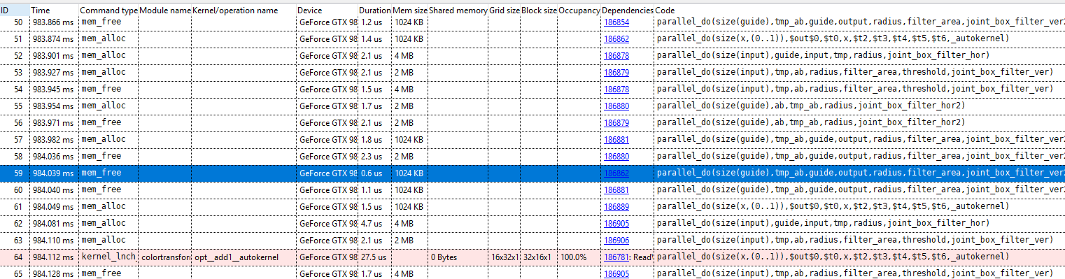
figure Figures/RedshiftProfiler-GPUEventsView.png

The following types of operations are listed:

```
mem_alloc
```
: a memory allocation operation
```
mem_free
```
: a memory deallocation operation
```
mem_transfer
```
: memory transfer operation
```
kernel_lnch_sync
```
: a synchronous kernel launch operation
```
kernel_lnch_async
```
: an synchronous kernel launch operation
```
device_func_call_sync
```
: a synchronous device function call
```
device_func_call_async
```
: an asynchronous device function call
```
sync_event
```
: a synchronization event
```
sync_event(global_sched)
```
(Hyperion engine only): indicates when the global scheduling algorithm was run (see multi-GPU programming guide for more information)

Notes:

In multi-GPU configurations, memory allocations of a single object may be listed multiple times, because an object may use memory of multiple GPUs.
Both synchronous and asynchronous kernel launches may be listed out of order with respect to other events. This is because the kernel start and duration times on the GPU are listed. Due to the nature of CUDA streams, the runtime may assume that an operation is finished at the moment a kernel function is launched, therefore a memory deallocation may occur even before the memory is used in a kernel function.

18.3.4 Timeline view

The timeline view now accurately depicts the kernel execution times and duration. In the following screenshot, it can be seen that both GPUs are (almost) fully utilized:

figure Figures/RedshiftProfiler-MultiGPUTimeLine.png

The mouse tooltips now also show a table containing the memory access information of the kernel function.

Oid: a unique object identifier (for a vector, matrix, user-defined object etc.)
Mode: the object access mode (
```
ReadOnly
```
indicates that the kernel function only reads the data,
```
WriteOnly
```
indicates that the kernel function only writes to the data,
```
ReadWrite
```
indicates both reading and writing).
Memory size: the amount of memory taken by this object.

This can be used to track down memory transfers, check the access mode (ReadOnly, WriteOnly) etc. By double-clicking on the object references, the operations to an individual object can be visualized in the GPU events view.

For

sync_event(global)

(which triggers a run of the global scheduling algorithm), the object reference that triggered the scheduling operation can be inspected:

figure Figures/RedshiftProfiler-GlobalSchedTooltip.png

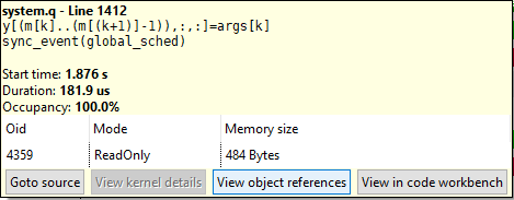
Note that a global scheduling operation can occur:

when the global command queue reaches its maximal capacity
when the CPU requires the result of an operation (for example, a kernel function returning a scalar value).

18.3.5 Kernel line information

When profiling a kernel with “collecting line information” enabled, execution information is displayed in the code editor:

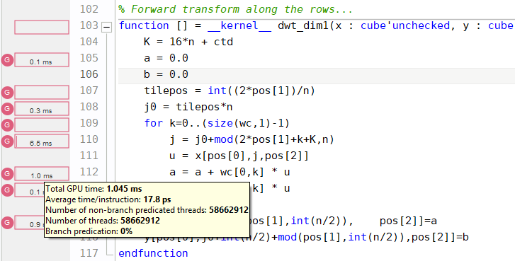
figure Figures/RedshiftProfiler-KernelLineInformation.png

Shown is the total execution time of running each line of the specified kernel on the GPU, as well as:

Average time per instruction: the total duration divided by the number of instructions (ignoring the parallelism)
Number of threads: the total number of threads that executed this instruction
Number of non-branch predicated threads: the total number of active threads (i.e., threads that are not disabled due to a false branch condition)
Branch predication: the percentage of threads that were disabled due to a false branch condition.

The kernel line information now allows to accurately identify bottlenecks within kernel functions, based on PTX to Quasar source code correlation. Note that due to compiler optimizations, the mapping from PTX to Quasar is not one-to-one. Therefore, the line information may not always correspond to the exact operation that was executed. To improve the correlation, the CUDA optimizations in the Program Settings dialog box can be disabled.

18.3.6 Kernel metric reports

Occupancy report

The occupancy report lists several parameters of the kernel function (block dimensions, data dimensions, amount of shared memory) and displays the calculated occupancy. Occupancy is a metric for the degree of “utilization” of the multiprocessors of the GPU.

Notes:

The calculated occupancy is not necessarily the real occupancy. By clicking the “single launch configuration” or “multiple launch configuration” buttons, the achieved occupancy can be calculated based on hardware metrics.
Occupancy is an indicator of performance, but a low occupancy does not necessarily results in a poor performance. It may happen for example that the function units of the GPUs are underutilized (e.g., due to a memory bandwidth bottleneck)
whereas the occupancy is maximal.

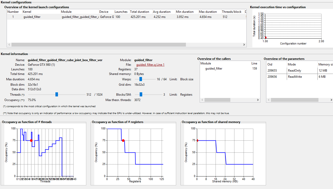
figure Figures/RedshiftProfiler-KernelReport1.png

The report displays the kernel execution time and subsequent analysis per launch configuration. A launch configuration is a set of parameter values, such as the grid dimensions, the block dimensions, the amount of shared memory being used). Because the performance of the kernel depends on the launch configuration, it is necessary to separate the measured profiling information according to the launch configuration.

In the bottom, the (theoretical) occupancy as function of respectively the number of threads/block, the number registers and the amount of shared memory is displayed. This indicates how occupancy can be improved:

The lower the amount of shared memory used by the kernel, the higher the occupancy will be. Of course, shared memory is required to mitigate the lower device memory bandwidth, therefore in practice a trade-off is always necessary.
Because the set of registers are shared between the different blocks, a lower number of registers may allow more blocks to run concurrently. Therefore, a lower number of registers generally leads to a higher occupancy.

However, the occupancy value is mostly indicates whether the launch configuration is selected to be “efficient” for the particular GPU. Unless the block dimensions are manually specified (e.g. via

parallel_do

{!cuda_launch_bounds max_threads_per_block=X}

, or

{!parallel_for blkdim=X}

), the runtime system uses in internal optimization algorithm to select the launch configuration that maximizes the occupancy.

In practice, an occupancy value of 50% (or even in many cases 25%) is sufficient to obtain maximal performance for the selected launch configuration. To gain more insights about the performance of a particular kernel, additional analysis is required.

Max. theoretical threads: calculated as the number of assigned warps × warp size × max active blocks, is the number of threads that is active on the GPU, after the warm-up phase of the kernel. If the occupancy value is smaller than 100%, check if the product of the data dimensions is smaller than max. theoretical threads. If this is the case, GPU multiprocessors are idle because the data dimensions of the kernel are too small.

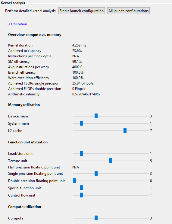
Overview compute vs. memory and function unit utilization

The compute vs. memory metrics are obtained by reading the hardware counters of the GPU. The following metrics are given:

Kernel duration: Indicates the duration of one single run of the kernel function in the selected launch configuration
Achieved occupancy: Shows the achieved occupancy of the kernel. The achieved occupancy is calculated based on the number of warps (and correspondingly threads) that have effectively been executed on the GPU. In the best case, the achieved occupancy is very close to the theoretical occupancy. When the achieved occupancy is significantly lower than the theoretical occupancy, the instruction scheduling issues may have occurred.
Warp execution efficiency: number of eligable warps per cycle compared to the total number of warps. An eligable warp is a warp that can be executed in the next cycle.
SM efficiency: The SM efficiency metric provides information about the effectiveness in issuing instructions.
Branch efficiency: The ratio of uniform control flow decisions over all executed branch instructions. When the branch efficiency is maximal, all threads within each warp take the same control path. A low branch efficiency indicates a poor performance due to branch divergence.
Average number of instructions/warp: Indicates the average number of instructions that were executed per warp.
Achieved FLOPs single/double precision: Gives the number of floating point operations per second (either single or double precision) that this kernel function achieves. It is useful to compare the achieved FLOPs with the maximally achievable FLOPs for the specific GPU (typically 5 TFlops or higher), although memory dependencies typically lead to significantly lower FLOPs.
Arithmetic intensity: a large value indicates that the kernel is compute-bound, while a small values signifies that the kernel is memory-bound (or stalls occur).

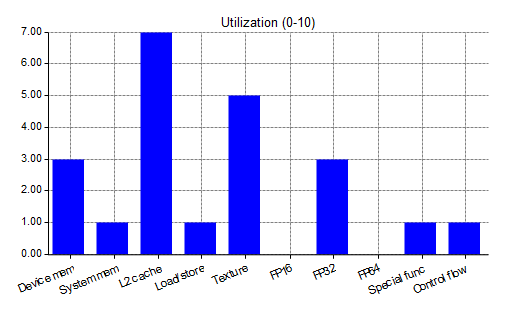
In addition, the utilization of the individual function units on a scale from 0 to 10 is displayed (the higher, the better).

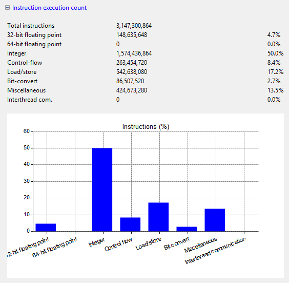
figure Figures/RedshiftProfiler-KernelReport2.png

figure Figures/RedshiftProfiler-KernelReport2b.png

Instruction execution count

The instruction execution count report shows the total number of instructions per type that were executed. Due to the presence of different function and computation units, maximal utilization can be achieved by balancing the operations. For example, when the number of floating point operations is much higher than the number of integer operations, it is useful to investigate whether some parts of the calculations can be done in integer precision.

Note: miscellaneous instructions are warp voting and shuffling operations.

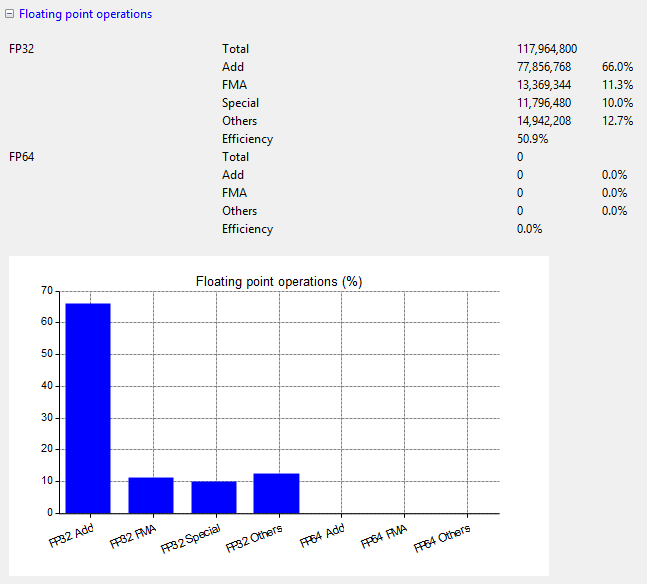
figure Figures/RedshiftProfiler-KernelReport3.png

Floating point operations

The floating point operations can further be categorized into:

Add operations
Multiply operations
FMA (fused multiply and add): the CUDA compiler combines add and multiply operations to improve the performance
Special: special mathematical functions (
```
sin
```
,
```
cos
```
etc.)
Others: other floating point operations (e.g. conversion between integer and floating point).

figure Figures/RedshiftProfiler-KernelReport4.png

Stall reasons

Issue stall reasons indicate why an active warp is not eligable.

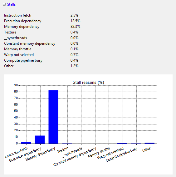
figure Figures/RedshiftProfiler-KernelReport5.png

The following possibilities occur:

Instruction Fetch: The next instruction has not yet been fetched.
Execution Dependency: An input is not yet available. By increasing the instruction-level parallelism, execution dependency stalls can be avoided.
Memory Dependency: too many load/store requires are pending. Memory dependencies can be reduced by optimizing memory requests (e.g., memory coalescing, caching in shared memory, improving memory alignment and access patterns).
Texture: too many texture fetches are pending
*__syncthreads*: too many threads are blocked by thread synchronization
Constant: A constant load leads to a constant cache miss.
Compute pipeline busy: Insufficient computation resources are available during the execution of the kernel.
Memory Throttle: Too many individual memory operations are pending. This can be improved by grouping memory operations together (for example, via the vector data types such as
```
vec(4)
```
).

Memory throughput analysis

The memory throughput analysis indicates the load/store and total throughputs (in bytes/second) achieved for the different memory units (shared memory, unified L1 cache, device memory and system memory), as well as the number of L2 cache operations and the hit rates of the L1 cache.

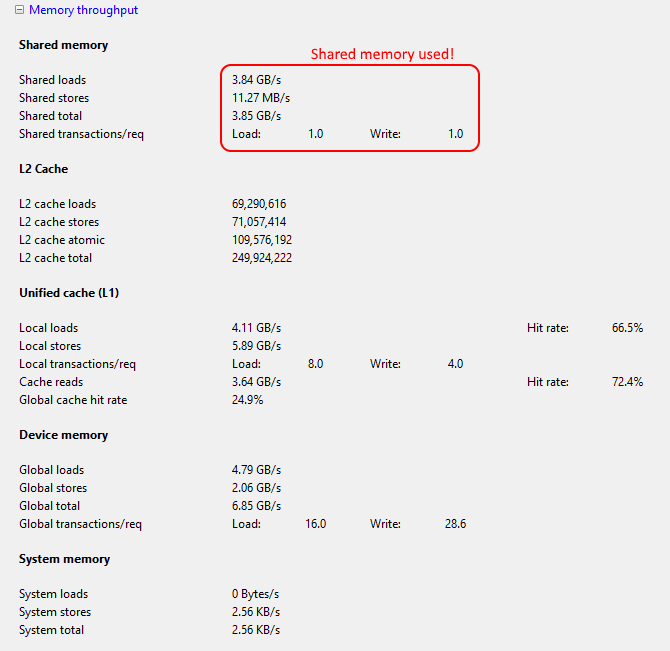
figure Figures/RedshiftProfiler-KernelReport7.png

Also shown are the average number of transactions per memory request. When the number of transactions per request is high, it may be beneficial to group the transactions (e.g., using vector data types such as

vec(4)

The best kernel performance is generally achieved by a good balance between operations using the different memory units. For many kernel functions, this practically means:

Use of shared memory whenever applicable: see the documentation on shared memory designators in Quasar
Use of texture memory, especially for readonly memory with a random access pattern.