Title: Tutorial 5: Variable inspection, profiling and optimization

Variable inspection, profiling and optimization

Profiling

To illustrate the Gepura development tools (in particular, the Quasar Redshift IDE), we will construct a random signal of length 64 and apply an averaging filter (for example, [0.2, 0.2, 0.2, 0.2, 0.2]) iteratively (1000 times) to the signal. Compare the run times for different signal lengths and check the GPU usage.

function [] = main()
    
    % number of iterations
    num_iter = 1000
    
    % define signal
    length = 64
    sig = rand(length)
    
    % define averaging filter (assumed to be of odd size)
    N = 2
    mask = ones(2*N+1,1)/(2*N+1)
    
    tic()
    for i=0..num_iter-1
        % filter the signal
        sig_new = zeros(size(sig))
        for m=0..length-1
            for k=-N..N
                sig_new[m] += mask[N+k] * sig[mirror_ext(m+k,length)]
            end
        end
    end
    toc()

    % show the filtered signal
    plot(sig_new)    
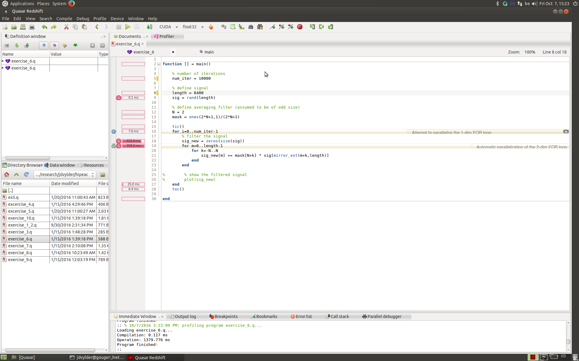
end 

Instead of just using tic-toc measurements we can get more detailed information about the execution time use the integrated profiler. Therefore, instead of running the program using the default ‘Run’ button, use the ‘Start Profiling’ option under the Profile menu. The IDE also shows the execution time at code level: The G-symbol indicates that this code line is executed at the GPU.

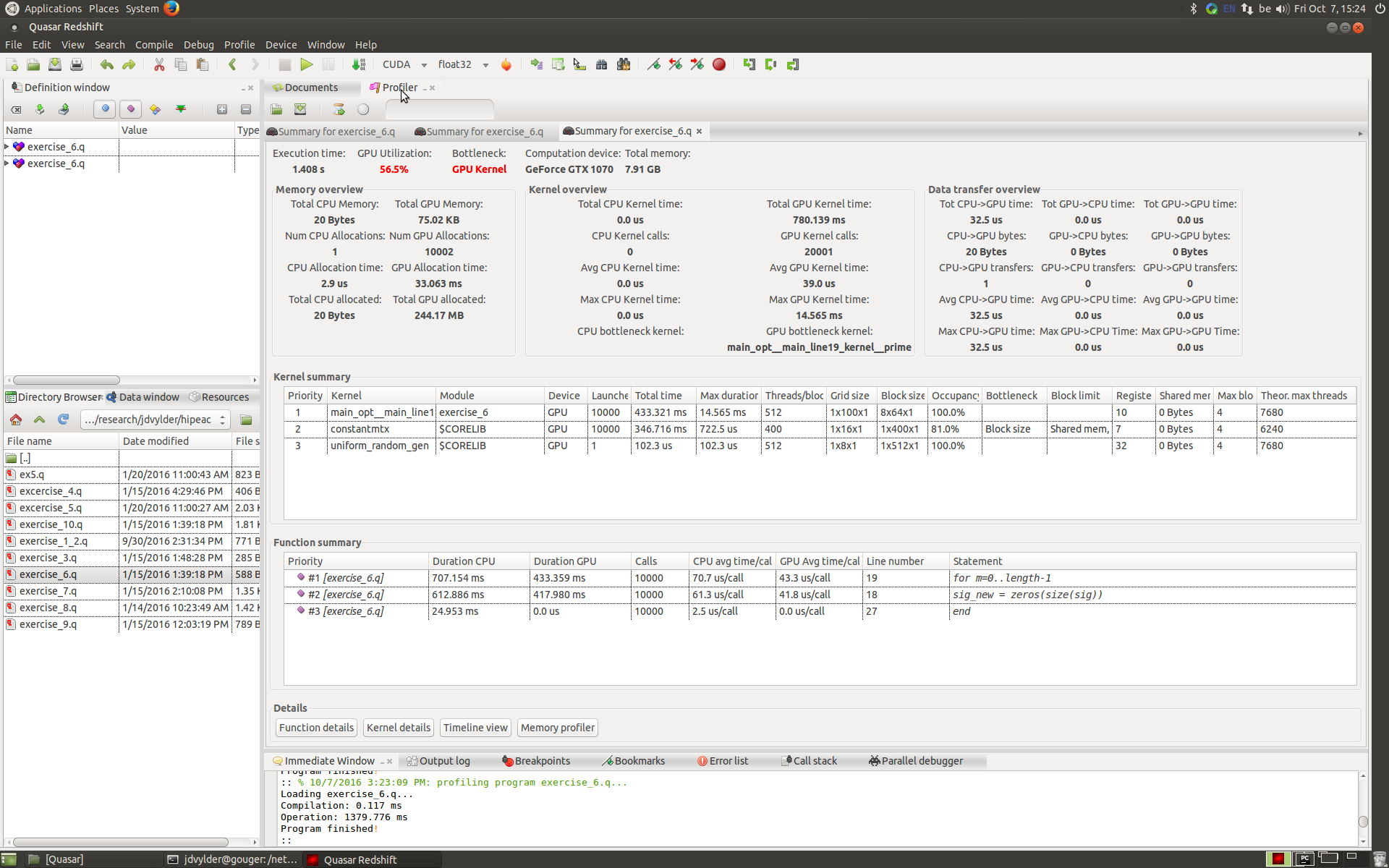
We will use the profiling result to isolate the highest priority bottleneck (in the kernel summary of the profiling result). Based on the observation that kernel opt_apply_mosaic clearly forms a bottleneck, we investigate the code and make the necessary changes to accelerate the algorithm. As it turns out, this kernel allocates a block of memory that it doesn’t really use (mask).

Therefore, the critical part of the code can be replaced by:

% define averaging filter (assumed to be of odd size)
N = 2

tic()
for i=0..num_iter-1
    % filter the signal
    sig_new = zeros(size(sig))
    for m=0..length-1
        for k=-N..N
            sig_new[m] += sig[mirror_ext(m+k,length)]
        end
    end
% normalization
sig_new /= (2*N+1)
end
toc()

Variable inspection

In order to explain the variable inspection in the Redshift IDE we will use the following code:

function [] = main()
    mask=[[1,2],[2,3]] %mosaic mask
    y = imread("image_mosaic.png")
    [M,N,K] = size(y)
    x_o = zeros(size(y))
    x_f = zeros(size(y))
    
    % display the raw mosaic data
    fig1=imshow(y)
    title("raw input data")
    
    % POCS algorithm
    tic()
    max_iteration=100
    for iteration = 1..max_iteration
        %this implementation swaps between using x_o and x_f as buffer
        %force data consistency
        parallel_do([M,N],x_o,y,mask,apply_mosaic)
        %force smoothness
        parallel_do([M,N],x_f,x_o,low_pass_filter)
        %force data consistency
        parallel_do([M,N],x_f,y,mask,apply_mosaic)
        %force smoothness
        parallel_do([M,N],x_o,x_f,low_pass_filter)
    end
    toc()
    
    %display the output
    fig2=imshow(x_o)
    title("full color image")
end

This program takes the raw input from a digital camera and constructs a full color image from it in an iterative fashion. The full program source code can be accessed here.

The current number of iterations is hard coded to a value that is far too high. By using the debugger we can investigate the evolution of the output x_o variable. First we set a breakpoint inside the loop. Once we the debugger breaks, we set a watch on the variable of interest (right click the variable name and click “add watch”). Then we click the red “probe” button in the data window to see live updates.

By manually iterating through the algorithm we can define a suitable iteration number, i.e., by clicking the start/continue button until the output result is a satisfactory full color image and then fix the algorithm to this max_iteration number, e.g., after 8 iterations we see little improvement. tip: you can mouse-over variables of different type while debugging to instantly glance their value.

Interactive debugging

We will create a small GUI (form) that shows the lena image on the left and an output image on the right. In the output image all values above a given value are set equal to this value. We will add a slider that allows a user to interactively set this saturation value.

import "Quasar.UI.dll"

function [] = main()
    img = imread("lena_big.tif")
    img_out = copy(img)

    frm = form("Quasar GUI demonstration")
    frm.move(150, 150)
    frm.width = 1500
    frm.show()



    slider_max = frm.add_slider("Maximum",255,0,255)
    slider_max.value = 255.0
    
    hl=frm.add_horizontallayout()
    disp1 = hl.add_display()
    disp2 = hl.add_display()



    function [] = update_display()
        img_out[:,:,:] = img .* (img < slider_max.value) + slider_max.value .* (img >= slider_max.value)

        f1=disp1.imshow(img,[0,255])
        f2=disp2.imshow(img_out,[0,255])
    end



    slider_max.onchange.add(update_display)
    
    update_display()
    end

Extra: make an adjustment such that when a user zooms in/out or pans the left image, that the same action happens on the output image. This can be done by adding a single line of code in the update_display function:

function [] = update_display()
    img_out[:,:,:] = img .* (img < slider_max.value) + slider_max.value .* (img >= slider_max.value)

    f1=disp1.imshow(img,[0,255])
    f2=disp2.imshow(img_out,[0,255])
    f1.connect(f2) % this line adds the desired functionality
end