Title: Quasar - Optimization Guide
Quick Optimization Guide
This document contains an introduction to optimization in Quasar. Generally, code that is written by hand is already reasonably fast: Quasar employs a variety of optimization techniques such as:
- Automatic generation of kernel functions for matrix expressions involving slice operations (
A[:,:,2] = B[:,:,c] .* sin(D)). - Automatic parallelization of for-loops
- Mappings onto shared memory (such as parallel reduction algorithms, parallel prefix sum algorithms)
- Reductions (for specifying alternative computation paths, such as
irealfft2(.)when calculatingreal(ifft2(.)).
Nevertheless, with proper knowledge, it is still possible to write poor-performing Quasar programs. As much as possible, the compiler will attempt to guide the user to write good code (by warnings e.g. labeled with the tag [optimization warning]).
The reasoning also differs from optimization in “traditional” programming languages such as C/C++, because there are more things going on behind the scenes. So the execution time of a Quasar program is often not directly related the number of statements/operations.
There are only five basic rules that the user needs to keep in mind:
Write parallel-code whenever possible. Either use for-loops with limited dependencies between the variables, or use the explicit parallel programming syntax (
parallel_do). Use{!parallel for}to ensure that the for-loop is parallelized (and not executed in interpreted mode). There are a number of patterns that are recognized and that can be parallelized efficiently (see Loop optimization patterns).Follow the compiler hints: for example, the hint “could not determine the type of output argument y”. Type inference (see Matrix data types and type inference) is very important in Quasar to generate highly performing code. In case the type of certain variables is not known, techniques such as automatic kernel generation / parallelization cannot be used.
Maximize data locality: use kernel functions that access (=reading/writing) the data only once instead of multiple times. It is better to have one kernel function that performs all the work than separate kernel functions that process the image in multiple stages. To this end, block-based processing approaches that make use of the shared memory are the most efficient. In some cases, a significant gain can be obtained (for example 4x faster), but again this may increase the complexity (see the Matrix multiplication example). The preferred solution in Quasar to reduce this complexity is by using generic programming patterns (see here).
Reduce the instanteneous memory footprint: minimize the amount of memory that is used at a given time, aim at kernel functions that process relatively small blocks of memory rather than huge blocks. Sub-divide large matrices into blocks. For example, when processing 3D data, it is generally more efficient to use a cell vector of 2D matrices, because: 1) whenever one slice is needed, only this slice needs to be transferred to the memory of the computation device, 2) smaller memory blocks may lead to less memory fragmentation (built-in memory compaction techniques are more efficient), 3) there is less risk of running out of device memory (for example processing 512^3 voxels on a GPU with 1 GB).
Don’t try to be smarter than the compiler. Most likely you are smarter than the compiler, however you may not be aware of what is happening behind the scenes. Avoid hand-optimization of programs by code duplication (such as loop-unrolling), substitution of values, pre-calculation of data (exceptions are however duplicate calculations, see below). These techniques work counter-productive as the maintenance of the code becomes more difficult. A common main principle is: the simplest programs should be the fastest ones. There are ways of passing hints to the compiler, e.g., using assertions, meta-functions or code attributes (pragmas), use them suitably.
From a language/runtime perspective, it is difficult to anticipate all possible use-cases, so there are situations in which the above techniques cannot easily be used. Therefore, some more hints:
In case there are intrinsic read/write dependencies between the elements of a for-loop that cannot easily be avoided, it is a good idea to switch to serial execution (
serial_do). Since recently this is done automatically (see Automatic serialization). Note that sequential algorithms are not necessarily non-parallelizable, for example, even for cumulative sums and infinite impulse response (IIR) filters, parallel implementations exist. These implementations use inter-thread communication, via shared memory or via warp shuffling. Consult the research literature to find a parallel implementation of a specific sequential algorithm.Solve the warning Warning: for-loop will be interpreted. This may cause performance degradation. When for-loop parallelization (or serialization) fails, there is still the possibility to run the for-loops in interpreted mode. However, some users have found that the for-loops can then become extremely slow (for example 50 seconds instead of 0.1 second). The reason is not that the Quasar interpreter is slow, but rather that there is a lot of internal management overhead by this approach. For example, when accessing an element of a matrix, the runtime system has to check every time whether the matrix is still in system memory, whether it was not changed in the meantime in the device memory etc. For-loop serialization/parallelization ensures that the code will be natively compiled (using C++ or NVCC), hence this way the program obtains the maximal performance benefits.
Balance the kernel load. The best situation is that one single
parallel_dooperation takes between 100ns-50ms:If the kernel loads are too small (e.g. <100ns), the computing device is not getting enough work to hide memory latencies. Moreover, there is extra overhead for the CPU and the driver in passing small chunks of work to the GPU.
If the kernel load is too big, the system may become irresponsive when the GPU is connected to the display device (for example GPU acceleration of the window manager). In Windows, there is even a watchdog timer that causes kernel functions that take longer than 5 seconds to reinitialize the device (reporting that the display driver has crashed).
There are techniques to mitigate the small kernel loads, see Kernel fusion.
To allow the compiler to perform advanced kernel optimizations, it is best to keep the kernel function definitions and the corresponding
parallel_dofunction call within the same scope. A common approach is to define a function that contains the kernel function as a sub-function and that launches this kernel directly. This way, the kernel function is only accessed within a local scope, making it much easier for the compiler to modify the kernel function and/or its parameters.Do not use too many small memory blocks (matrices, class objects such as linked list nodes). Small blocks can lead again to memory fragmentation and even though individual memory transfer operations are be batched internally in the Quasar runtime, the most efficient approach is still the transfer of one contiguous block of memory. In case many small blocks are necessary, consider using vector/array types that store these blocks in a contiguous fashion. For example
vec[my_type]rather thanvec[^my_type].From the above, one could conclude that data structures like linked-lists or trees are not very efficient in Quasar. This is not true - the structures need to be implemented with care and according to the above guidelines. Therefore: a linked list could be implemented as follows:
 type linked_list_node : mutable class
     index_prev : int
     index_next : int
     value : scalar
 endtype

 type linked_list : vec[linked_list_node]
Note that this requires pre-allocation, i.e. having an idea of the size of the list in advance.
Differences between CPU and GPU devices
Threads. CPUs typically provide a low number of threads, while for GPUs the number of threads can be more than 1024. Note that in contrast to the CPU, the GPU threads are light-weight. If the GPU must wait on one group of threads, it simply begins executing work on another group of threads. Because the registers are already allocated in advance for all active threads, no state switching or swapping of registers is required when switching between GPU threads. Resources remain allocated to each thread until it completes its execution. Correspondingly, CPU cores minimize latency for one or two threads at a time each, whereas GPUs are able to handle a large number of concurrent, lightweight threads in order to maximize throughput.
One iteration of a parallel_do statement (or one single kernel invocation) leads to the creation of one single thread. For efficiency, the CPU computation device uses OpenMP in a block-based fashion similar to the CUDA blocks to avoid the state switching and the construction of the heavy weight CPU threads.
Throughput. Because of the many parallel threads, a GPU-implementation can be up to 10x-20x faster than a hand-optimized C/C++ implementation that runs on the CPU. Because many operations e.g. on high-definition television images require less than 5ms for processing, the Quasar programs on the GPU are well suited for real-time video processing.
High throughput of the GPU is achieved by hiding memory latency, provided that there is sufficient parallelism (i.e. the data size is large enough, typically > 10000). To maximize throughput, the memory architecture of the GPU needs to be taken into account (see Memory).
On the other hand, CPU implementations can be vectorized and take advantage of SIMD instructions of the processor. This is also supported by Quasar.
Memory. CPUs and GPUs have distinct memory spaces. This means that the Quasar runtime system needs to keep track of which memory is in CPU/or GPU memory, whether it was last modified in which memory. The runtime also needs to transfer the data from/to GPU at the proper times. There are a number of techniques being used to ensure that this is done in an optimal way (these techniques work in a transparent way - the user does not need to be aware of this):
The use of DMA (Direct Memory access) - this is a technique that allows memory of the CPU to be mapped onto the address space of the GPU, so that the GPU can directly read from the CPU memory. This technique is very fast when the memory is only read once on the GPU (the so-called streaming mode).
Look-ahead mode (Concurrent kernel execution mode) - in this mode, the CPU runs asynchronously from the GPU. This also means that while the GPU is still processing its data, the CPU is already looking forward and planning future memory transfers. If the GPU supports it (and most recent devices do), the memory transfers are scheduled in parallel with the kernel execution. So this means that the memory transfers can be nearly for-free in some cases.
Minimization of memory transfers - the runtime only transfers data to the GPU if the subsequent processing steps are most efficient on the CPU. When only a small kernel need to be executed, this kernel is scheduled to run on the CPU, avoiding the memory transfer. Programs that require to run multiple kernels need to make sure that the data remains on the GPU. While in CUDA/OpenCL this requires a lot of manual work, this is done in a transparent way.
GPU memory types - the GPU has several memory types (global memory, shared memory, constant memory, texture/surface memory) that all have their own bandwidth and latency. In some cases it is beneficial to even mix different memory types (e.g. one variable is stored in constant memory, another variable in texture memory etc.).
There are a number of high-level settings that allow to control the memory management system. It is for example possible to indicate that the program is memory-hungry and tends to use all the available GPU memory. By default, the runtime system only allocates what is needed, leaving some memory free for other applications (or other Quasar processes). Some more information can be found in CUDA Memory management enhancements.
Host function level optimization
Several techniques can be used to optimize host (i.e. non-kernel/device) functions. Note that these techniques often reduce the readability of the code.
Uninitialized memory allocation. Memory allocation using the function
zerosinternally performs an extra step in which the CPU (or GPU) memory associated to the matrix is cleared. This extra step takes for large matrices (e.g.2000x4000) about 1 ms, but can be avoided when a subsequent operation will overwrite the entire matrix. This can be accomplished using the functionuninit.An example is the following kernel function:
 A = uninit(2160,3840,3)
 parallel_do(size(A), __kernel__ (pos : ivec3) -> A[pos] = 2.0)
The function
uninitperforms uninitialized memory allocation, which is similar to unitialized memory on the stack or heap in C/C++. Note: in the first phase of the development, it is recommended to use the functionzeros, in order to switch in a later phase touninit(when it is certain that all kernel functions work as ‘intended’). This is to avoid unexplainable oddities in the results due to the abuse of the uninitialized memory.Eliminate redundant calculations: obviously, the less work that has to be done, the lower the computation time. Consider the following loop:
 function [] = __kernel__ box_filter_hor(x : cube'mirror, y : cube'unchecked, r : int, pos : vec3)
     sum = 0.
     for i=-r..r
         sum = sum + x[pos + [0,i,0]]
     endfor
     y[pos] = sum
 endfunction
 parallel_do (size(x_in), x_in, x_out, r, box_filter_hor)
 parallel_do (size(y_in), y_in, y_out, r, box_filter_hor)
 z = (x_out + y_out) / 2
The code performs a horizontal box filtering of two inputs and finally averages the results. Here, one of the filtering steps can be avoided by exploiting the linearity of the convolution (i.e. (
a * h + b * h = (a + b) * h)). This leads to the following (about 2x faster) implementation:function [] = __kernel__ box_filter_hor(x : cube'mirror, y : cube'unchecked, r : int, pos : vec3) sum = 0. for i=-r..r sum = sum + x[pos + [0,i,0]] endfor y[pos] = sum endfunction z_in = 0.5 * (x_in + y_in) parallel_do (size(x_in), z_in, z, r, box_filter_hor)Kernel function merging: often many kernel functions perform relatively simple operations (for example, multiplying two matrix elements, applying a point-wise function, box filtering). It turns out to be more efficient to have a small number of kernel functions that relatively perform a lot of work rather than a large number of kernel functions performing each a little bit of work. For example:
 function [] = __kernel__ box_filter_hor(x : cube'mirror, y : cube'unchecked, r : int, pos : vec3)
     sum = 0.
     for i=-r..r
         sum = sum + x[pos + [0,i,0]]
     endfor
     y[pos] = sum
 endfunction
 parallel_do (size(x_in), x_in, x_out, r, box_filter_hor)
 parallel_do (size(y_in), y_in, y_out, r, box_filter_hor)
The two parallel loops (over
x_inandy_in) could better be replaced by:function [] = __kernel__ box_filter_hor2(x_in : cube'mirror, y_in : cube'mirror, x_out : cube'unchecked, y_out : cube'unchecked, r : int, pos : vec3) sum1 = 0. sum2 = 0. for i=-r..r sum1 = sum1 + x_in[pos + [0,i,0]] sum2 = sum2 + y_in[pos + [0,i,0]] endfor x_out[pos] = sum1 y_out[pos] = sum2 endfunction parallel_do (size(x_in), x_in, y_in, x_out, y_out, r, box_filter_hor2)or even better, by using fixed-length vectors:
 function [] = __kernel__ box_filter_hor2(x_in : cube'mirror, y_in : cube'mirror,
      x_out : cube'unchecked, y_out : cube'unchecked, r : int, pos : vec3)
     sum = [0., 0.]
     for i=-r..r
         sum = sum + [x_in[pos + [0,i,0]], y_in[pos + [0,i,0]]]
     endfor
     [x_out[pos], y_out[pos]] = [sum1, sum2]
 endfunction
 parallel_do (size(x_in), x_in, y_in, x_out, y_out, r, box_filter_hor2)
Of course, this optimization is only valid when
size(x_in) == size(y_in). The motivation for this optimization technique is memory access latency hiding: typically for these type of functions, the memory accesses are the primary bottlenecks. By putting multiple memory accesses closely together, the latency of one memory access can be hidden by the latency of another memory accessVector-based processing/scalar processing:
For image processing algorithms, it is possible to either threat all color components together in a fixed-length vector (
vec3), or to process each color component separately.See the example below, for the
circshiftfunction:function y = circshift_vector(x : cube, d) % Vector-based processing function [] = __kernel__ process_RGB(x : cube'circular, y : cube'unchecked, d : ivec2, pos : ivec2) y[pos[0],pos[1],0..2] = x[pos[0]+d[0],pos[1]+d[1],0..2] endfunction y = uninit(size(x)) parallel_do(size(x,0..1),x,y,d,process_RGB) endfunction function y = circshift_scalar(x, d) % Scalar processing function [] = __kernel__ process_RGB(x : cube'circular, y : cube'unchecked, d : ivec2, pos : ivec3) y[pos] = x[pos + [d[0], d[1], 0]] endfunction y = uninit(size(x)) parallel_do(size(x),x,y,d,process_RGB) endfunctionFor similar reasons as with the kernel function merging technique, the vector-based processing turns out to be to most efficient (about two times as fast).
The vectorized approach is even recommended by NVidia. See for example: http://devblogs.nvidia.com/parallelforall/cuda-pro-tip-increase-performance-with-vectorized-memory-access/.
For-loop parallelization: it is important to make sure that the for-loops can appropriately be parallelized (or serialized) by the compiler. This way, the loops are entirely executed on the computation device (e.g. GPU). It is necessary that the types of all variables are known at compile-time. Whenever possible, the compiler will try to obtain these types from the context (for example, based on the caller information via a function specialization, or by inlining functions with unspecified types). In the following example, the for-loop can be parallelized, despite the function
fhaving unknown (dynamic) parameter types:img = imread("lena_big.tif")[:,:,1] function [] = my_func(f : [(??,??)->??]) {!parallel for} for m=0..size(img,0)-1 for n=0..size(img,1)-1 img[m,n] = f(2, img[m,n]) % will be inlined endfor endfor endfunction fn = (a, b) -> a + b my_func(fn)
Kernel/device function level optimization
There are a number of simple optimization hints that you can use inside a __kernel__ or __device__ function.
Integer types. Whenever possible, use the type
intinstead ofscalar, for example by defining constants like 1, 2, 3, rather than 1.0, 2.0, 3.0 etc. To further gain performance, promote kernel argument types tovec[int],mat[int],cube[int](even though this is not recommended for rapid-prototyping). Note that the Quasar compiler attaches importance to the presence of the decimal point. In case a decimal point is missing, the corresponding variable type is integer, otherwise the variable type is scalar.Memory coalescing. Very often, different threads require access to different elements of a matrix. When the different elements of this matrix are stored contiguous (i.e. in subsequent indexes), the GPU hardware is able to group up to 16 (or 32) of these memory loads together (=coalescing), rather than requiring 16 (or 32) different load operations. Coalescing significantly reduces the memory access times, often with factors of 4 or more. By default, Quasar is designed so that algorithms will automatically use coalescing: for example:
contrast_enhancer = __kernel__ (pos : ivec2) -> im[pos] = 2 * im[pos]However, if you would transpose the matrix for some reason:
contrast_enhancer = __kernel__ (pos : ivec2) -> im[pos[1],pos[0]] = 2 * im[pos[1], pos[0]]Memory coalescing would suddenly not be possible: the different elements are no longer 1 position apart, but 1 row. In case of an uncoalesced access, the compiler gives a warning:
Warning: uncoalesced access to variable
imwhile a preliminary analysis shows that a coalesced access is possible.struct of vectors vs vectors of arrays. Suppose you want to stores structured data in a vector:
 type point : class
     x : scalar
     y : scalar
     radius : scalar
 endtype
 type point_vec : vec[point]
Similar as in point 2, the vector
point_vecdoes not enable coalescing on a GPU. Instead, for the best performance, it is recommended to use structs of vectors:type point_vec : class x : vec y : vec radius : vec endtypeInteger division. By default, the result of the division of two integer values is
scalar. This is to avoid confusion, as the variable types are obtained through type inference, so the inferred variable types may be not very obvious to the programmer (even though Redshift provides information when hovering with the mouse over the variable. Nevertheless: to compute the true integer division, it suffices to apply theintfunction to the result:result = int(a/b)It might be not very obvious, but internally, the operation
int(./.)is optimized into integer division.Floating point division: floating point division is notoriously slow, although in many cases a full precision is not required. Quasar provides the functions
div_approx(a,b)to calculate an approximate division of variablesaandb. For calculating the reciprocal in casea==1, the following functions are available:rcp_rn: calculate1/a, round to the nearest floating point numberrcp_ru: calculate1/a, round up to the next floating point numberrcp_rz: calculate1/a, round down towards zero
Bit-shifting operations. In case the goal is to multiply/divide integers by powers of two, such as (assume
binteger):a_divided = int(a/2^b) a_multiplied = int(a*2^b)This can be implemented more efficiently using bitshifts:
 a_divided = shr(a,b)
 a_multiplied = shl(a,b)
Here,
shrdenotes a right bitshift, whileshlindicates a left bitshift. Note that in future versions, this may be done automatically by the compiler.Use Vectors with explicit length annotation (
ivec2,cvec3,vec4, …). Arithmetic using the vector-types for which the length is known at compile-time can further be optimized. For example, the vectorizing compilers (such as LLVM, GCC, Intel C/C++) can then generate SIMD instructions more easily. For x86/x64 targets, usevec4,ivec4,cvec2over other vector lengths, to obtain the benefits of SSE instructions. Note thatvecX,ivecXandcvecXtypes are by-reference types, likevec,mat,cube.Note that the current length that can be specified for
vecX,ivecXandcvecXtypes is limited to 64.Use Matrices with explicit size annotations (
mat(2,2),cube(2,3,2)). Similarly to vectors with explicit length, matrices can also be represented in vector-types. For this purpose, the dimensions of the matrix need to be known at compile-time. SIMD instructions can be applied for example on variables of typemat(2,2).Use shared memory whenever possible. However, only use shared memory when the same locations are being read/written multiple times (otherwise there is no benefit). Avoid bank conflicts.
When using shared memory, make sure that the upper bound for the required amount of shared memory can be computed at compile-time. You can do this by inserting assertions on the arguments passed to the function
shared(.). This way, the multi-processor may process several blocks simultaneously, whereas otherwise it must be assumed that the kernel function used the maximum amount of available shared memory (which only allows one block/multiprocessor). For example:assert(nthreads<16) A = shared(nthreads, 256) % The compiler will find that maximally 16K is needed in single-precision floating point mode.Ideally, the amount of shared memory used by a kernel function should be the maximum amount of shared memory divided by the number of blocks the GPU can handle in parallel (=the number of multi-processors). For 32K shared memory and 8 multiprocessors, this is 4K (or 1024 single precision floating point numbers). Often, this corresponds to the number of threads within one block.
When possible, use Warp shuffling operations as an alternative to shared memory
Warp shuffling operations allow threads to access data from other threads within the warp (i.e. a group of 32 adjacent threads). See Quick Reference Manual on the topic “Cooperative Groups and Warp Shuffling functions” on how to use warp shuffling. The Quasar compiler will also generate code using warp shuffling instructions in some cases (see Parallel reduction transform).
Avoid different execution paths along threads inside one block. This may cause so-called thread divergence - the block is finished when all threads for this block have been finished. In CUDA, instructions execute in warps of 32 threads. A group of 32 threads must execute (every instruction) together. Control flow instructions (
if,match,repeat,while) can negatively affect the performance by following different execution paths. Then the different execution paths must be serialized, because all of the threads of a warp share a program counter. Consequently, the total number of instructions executed for this warp is increased. When all the different execution paths have completed, the threads converge back to the same execution path.To obtain best performance in cases where the control flow depends on the block position (
blkpos), the controlling condition should be written so as to minimize the number of divergent warps.For example, instead of
if input[pos] > 0
  accumulator_pos[pos] = input[pos]
  accumulator_neg[pos] = 0
else
  accumulator_pos[pos] = 0
  accumulator_neg[pos] = input[pos]
endif
Consider a version which has no control flow.
value = input[pos]>0
accumulator_pos[pos] = value
accumulator_neg[pos] = x - value
The above transformation can also be obtained by enabling the branch divergence reduction kernel transformation:
{!kernel_transform enable="branchdivergencereducer"}Avoid recomputation. Suppose that you need the value for
A[u,v,0]at several places in the code, it is often more efficient to store the value in a temporal variable (which saves several read access to the RAM memory) - the temporal variables are usually stored in the device registers. The reason that the Quasar compiler currently does not optimize automatically duplicate read accesses, is that concurrency may occur:phase = theta[pos] [x, y] = [cos(phase), sin(phase)] syncthreads phase = theta[pos] + pi/4 % Another thread may have changed theta[pos] [x2, y2] = [cos(phase), sin(phase)]In future versions, the compiler may be able to exploit the
'constmodifiers in order to perform the temporal variable substition automatically.Avoid atomic operations on the same memory location. While it may be convenient to incrementally add numbers to a matrix, using
A[pos] += x, an atomic add operation is used internally for implementing the+=operator. This is mainly for avoiding data races between parallel threads.- In case the atomic add does not cause a data race, the atomic operation is relatively fast.
- In case the atomic add is performed on a local variable (and hence completely free of races), the compiler automatically replaces
+=by the non-atomic version. - When the atomic add does cause a data race, the performance can be really poor: the operations will then be performed sequentially, and the program will not perform faster than a direct CPU implementation.
The solution is then to use the parallel sum algorithm (see Reference Manual) instead. The sample
atomicadd_vs_parallelsum.qillustrates the necessity of this enhancement. On a Geforce 435M, 100 atomic adds on an image take 531ms, while using the parallel sum algorithm it is only a mere 73ms. This is a speed-up of a factor 7.2 (!)syncthreads. When
syncthreadsis called by one thread, it should be called by all other threads in the block, otherwise either the performance is degraded or the result is undefined! This is particularly of importance when callingsyncthreadsinside anif/for-construction.Hardware texturing units (HTU). Consider the use of hardware texture mapping (
hwtex_nearestandhwtex_lineartype modifiers) when there are a lot of irregular data access. Hardware texture units have built-in support for certain forms of boundary checking (in particularcircular,mirrorandclamp) and even for linear interpolation. Moreover, they have internal caches (6-8 KB/multi-processor and are optimized for 2D or 3D localized accesses. In many circumstances, the HTU’s further improve the performance up to 2x-3x. Even for nearest-neighbor interpolation with no special boundary accessing modes, the speed-up is usually 10-30%.As an example, consider image scaling using linear interpolation:
function [] = __kernel__ interpolate_hwtex(y:mat, x:mat'hwtex_linear, scale:scalar, pos:ivec2)
    y[pos] = x[scale*pos]
endfunction
The HTU here takes care of both the linear interpolation and the boundary checking. Note that the
hwtex_nearestandhwtex_linearcan only be used for reading (not for writing)!Kernel function output arguments. Quasar offers kernel function output arguments as a convenience feature, for example when calculating a single number:
  function [y : int] = __kernel__ my_kernel(pos : ivec2)
      if A[pos] > 127
          y += 1
      endif
  end
  num = parallel_do(size(A), my_kernel)
The problem here is not the fact that all threads perform an atomic assignment
y+=1: the parallel reduction transform will actually optimize this pattern, however, the assignment[num, z] = ...causes the result to be read immediately in order to store the values in variables. This inevitably leads to a transfer to the CPU and a device sychronization. To fix this issue, simply allocate a vector of length 1 and pass this vector to the kernel function.function [] = __kernel__ my_kernel(y : vec[int], pos : ivec2) if A[pos] > 127 y[0] += 1 endif end num = vec[int](1) parallel_do(size(A), num, my_kernel)Then the result will be read out only at the moment it is needed on the CPU. The parallel reduction optimization will still be applied.
Avoid (or limit) matrix creation/allocation inside for-loops
When possible, Quasar will store arrays (vectors, matrices, …) with a known fixed size (such as vec4, cvec6, mat(3,4)) into the registers of the device. The register accesses are significantly faster than the global memory accesses, which gives a lot of computational benefits. However, assigning registers is only possible when the array size is known in advance and the number of elements <= 64.
However, for vectors for which the length can not be determined at compile-time, the vectors cannot be stored into the device registers, simply because the vector length is not known. The vector data needs to be stored elsewhere, and that is in the dynamic kernel memory. The dynamic kernel memory is (for GPU computation devices) a part of the global memory of the GPU, hence the access time is significantly slower than in case of the device registers. In addition, the dynamic allocation bears additional overhead due to atomic access operations that ensure that each thread gets a different memory block. For this reason, it is generally better to avoid using the dynamic kernel memory whenever possible (especially when an implementation is possible without dynamic kernel memory). Therefore, the compiler will optionally generate a performance warning when dynamic kernel memory is being used automatically.
Of course, there are many situations in which it is not possible to assign fixed-length vectors. For example, a common scenario is the creation of matrices inside for-loop. Consider the following implementation of a linear filter:
for m=0..size(x,0)-1
    for n=0..size(x,1)-1
        % Extract a sub-block
        x_sub = x[m+(-M..M), n+(-M..M)]   % STEP 1

        y[m,n] = sum(x_sub.*mask)  % STEP 2
    endfor
endfor
The problem here is that - since M is not known at compile-time, step 1 dynamically allocates memory inside the for-loops. Using dynamic memory comes at a cost: when there are K threads, and each thread allocates a large matrix of size N. Then this requires KN global memory accesses (which are usually very expensive). In situations when registers could be used (for example using vec1, vec2 types)
There are often different solutions possible to avoid using dynamic memory:
By setting M as a constant
It suffices to specify
M : int'const = 1, then the compiler will determine that the dimensions ofx_subare 3x3. Note that the modifier'constis important here, it allows the compiler to perform the substitutionM=1by avoiding temporary variables, calculating the result directly:
for m=0..size(x,0)-1 for n=0..size(x,1)-1 y[m,n] = sum(x[m+(-M..M), n+(-M..M)].*mask) % STEP 1 & 2 endfor endfor
By the automatic kernel generator, the
sum()operation will be expanded into essentially the following loop, which is free of memory allocations.{!parallel for} for m=0..size(x,0)-1 for n=0..size(x,1)-1 sum = 0.0 for k = -1..1 for l = -1..1 sum += x[m+k, n+l] .* mask[1+k,1+l] endfor endfor y[m,n] = sum endfor endforNote that the
{!parallel for}attribute is actually not required here, it just ensures that the parallelization will work (giving a compiler error message if it doesn’t), so that the program will not accidentally run in interpreted mode.vector creation inside a loop:
Use:
 type pointcloud : cube
 data = pointcloud(256, 256, 3)
Rather than:
 type pointcloud : mat[vec]
 data = pointcloud(256, 256)
 for k=0..size(data,0)
     for l=0..size(data,1)
         data[k, l] = zeros(1, 3)
     endfor
 endfor
In the last example a fixed length vector is used, however the assignment to an element of
mat[vec]would cause the fixed length vector to be converted to a dynamic length vector. Themat[vec]data structure does not impose restrictions on the vector lengths of its elements: each element is allowed to have a different length.One could think that a simple solution is to use a fixed-length vector:
type pointcloud : mat[vec3]However, the above type is currently mapped onto
mat[vec]during code generation (which means that the length information is lost). Even though this may be fixed in future versions of Quasar, better alternative is to use data types with partially known dimensions:type pointcloud : mat[:,:,3]
use stack memory
An alternative to dynamic memory is stack memory. Stack memory can be used whenever the allocation size can be determined at compile-time. To enable stack memory to be used within a loop or kernel function, it is sufficient to place
{!kernel memorymodel="stack"}as in the following example:
 for i = 0..n-1
     {!kernel memorymodel="stack"}
     max_stack_size = 16
     stack_top = 0
     stack = zeros(max_stack_size)

     % Push an index to the stack
     if stack_top < max_stack_size
         stack[stack_top] = index
         stack_top += 1
     endif
 endif
On the GPU, the registers and the global memory (when necessary, this is called register spilling) is used as storage for the matrix variables. This provides less overhead than the dynamic memory subsystem. In the best case, the data is stored in the registers, in the worst case in global memory (which is the same as for dynamic memory).
Functions triggering dynamic kernel memory usage
When writing higher-level code, the programmer often does not think about implications of allocating data types with arbitrary sizes. On the one hand, this is a good thing, since the data sizes (vector lengths, matrix dimensions) can be considered to be implementation details, but on the other hand this may have some performance and usage impact when executing on accelerators such as GPUs.
Even though the compiler avoids generating code based on dynamic kernel memory and (e.g., by merging several functions together), in some cases, dynamic kernel memory allocations cannot be bypassed. Generally speaking, this is the case when the calculated result is an array for which the size cannot be determined at compile-time.
The Quasar compiler will generate warning messages such as “Kernel/device function consumes dynamic kernel memory, which may negatively impact the performance. Check if dynamic memory can be avoided here”. In our experience, avoiding dynamic kernel memory whenever a static alternative exists can speed up the GPU kernel by a factor 10 or more.
Some examples are listed below (note that the following list does not give a definitive answer - depending on the context, dynamic memory may be used or not. It is best to inspect the compiler warnings):
- Vector or matrix allocation functions
zeros(N),uninit(M,N)whereNandMcannot be determined to be constant at compile-time - Output parameter types of device functions (a device function returning
vec,matetc.) - The matrix sizing functions
reshape,squeeze,shuffledims,transpose,repmat,shuffledims, for which the output dimensions cannot be determined at compile-time (or the number of elements >= 64). - The matrix-vector or matrix-matrix multiplication operation
- The matrix slice indexer
:(in general, a fixed length vector can be obtained by specifying ranges, such as:A[u,v,0..2], similarly a fixed sized matrix will also work without dynamic memory allocationA[u,v+(0..2),0..2]).
Automatic use of dynamic memory is allowed for convenience, but improper use of dynamic memory may degrade the performance, for three reasons:
- When using dynamic memory, the compiler is often no longer able to determine the size of the result (e.g. the vector length), leading to additional variables that need to be stored in the dynamic memory. An exception are the cases in which one of the operands has a fixed size, for example for the addition
vecX+vec, for which the result is guaranteed to bevecX. - As already mentioned, access to the dynamic memory is significantly slower than access to the GPU shared memory or the device registers.
- There are extra (invisible) costs involved in managing dynamic memory blocks (allocation, de-allocation and reference counting). Although generally small, when large number of dynamically allocated variables are used, the cost may be severe.
Tips for avoiding dynamic kernel memory inside kernel/device functions or parallel loops: * Use fixed-length vectors (e.g., vec12) over vectors with unspecified length (e.g., vec). * This also holds for the output parameters of device functions. * Avoid data types with recursion, for example vec[mat], vec[cube]. When the dimensions of the components are equal, use a higher-dimensional data type instead (for example, cube or cube{4}). * Often, pre-allocating the memory (from the calling host function) may totally avoid the problem.
Whenever possible, the Quasar compiler may take aggressive measures to avoid dynamic kernel memory automatically, for example, by optimizing it out entirely.
Advanced compiler optimizations
This chapter gives an overview of the optimizations performed by the Quasar compiler; and some means for the programmer to interact with the compiler (e.g., giving feedback or triggering additional new optimization steps). The optimizations have been continuously tested on a large body of test Quasar programs; however, new optimizations may be expected in the future and this document will also be updated accordingly.
Overview
The compiler processes Quasar code using an entire pipeline of front-end optimization passes. An example of such a pipeline for generating GPU and CPU specific code is shown in the picture below. Therefore it is useful to discuss the processing steps and how they improve performance. Some optimization passes can only be activated through certain programming patterns, or by explicit hints by the user (this is to avoid that an optimization phase would negatively impact performance).
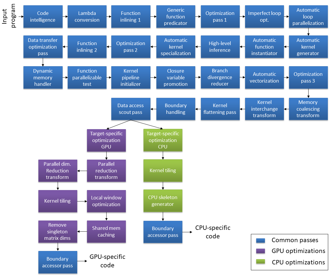
(Note: this picture is the current state as of July 2017, the exact blocks and order may change in future version)
In addition, the back-end compilers (e.g. GCC, NVCC) may apply their own optimization phases separately. We are not doing double work: the Quasar optimization passes are generally on a higher language abstraction level than the level that a C++ or CUDA compiler has access to. Therefore the two approaches (front-end and back-end optimization) are complementary.
There are two types of passes:
- Function transforms: which work on functions as a whole
- Kernel transform: which deal with kernel/device functions. This may also include making changes to the
parallel_do()andserial_do()function calls that launches the kernel function.
Some of the passes can be enabled or disabled manually from the code. An overview is given below.
Enabling/disabling function transforms:
| Function transform | Code attribute |
|---|---|
| Automatic kernel generator | {!function_transform enable=“kernel_generator”} |
| Imperfect loop optimization | {!function_transform enable=“imperfectloop”} |
| Eliminate common subexpressions | {!function_transform enable=“eliminate_common_subexpr”} |
Enabling/disabling kernel transforms:
| Kernel transform | Code attribute |
|---|---|
| Parallel reduction transform | {!kernel_transform enable=“parallel_reduction”} |
| Parallel dimension reduction transform | {!kernel_transform enable=“parallel_dimension_reduction”} |
| Kernel tiling | {!kernel_transform enable=“kernel_tiling”} |
| Memory coalescing transform | {!kernel_transform enable=“memcoalescing”} |
| Branch divergence reducer | {!kernel_transform enable=“branchdivergencereducer”} |
| Loop flattening | {!kernel_transform enable=“loop_flattening”} |
Code intelligence
The code intelligence pass performs various preparation steps for subsequent optimizations. The most important step the type inference, which derives the types of variables with unknown type from the types of variables with known type. For this purpose, for function calls, the types of the output parameters may be recalculated based on available information on the input parameters.
The compiler employs a hybrid static and dynamic typing system, in the sense that as many types as possible are statically determined at compile-time. This benefits optimal code generation for CPU and GPU. When generating kernel/device functions it is even required that the involved parameter and variable types are statically determined (resulting in a compiler error if this is not the case). The main motivation for this is that it does not make much sense to implement dynamic typing on an accelerator device. These issues can then fairly easily be resolved by the user by explicitly indicating the type of some of the variables.
Finally, the code intelligence step also detects inlineable functions (to be inlined during the function inlining pass) and updates the truth-value system iteratively based on new information available in each statement. Other transform passes can then exploit the gained knowledge in order to generate more efficient code.
Lambda conversion transform
The lambda conversion transform is a mostly syntactic transform that translates lambda expressions into regular functions. This allows lambda and kernel functions to be handled within the same compilation framework (note that other than syntax and overloading differences regular functions and lambda expressions in Quasar are fairly similar).
Function inlining transform
The function inlining transform inlines functions that are annotated with {!auto_inline} and also function calls with $inline() being set. For example: the following function will always be inlined:
function [x,y] = __device__ mysincos(theta)
    {!auto_inline}
    [x,y] = [sin(theta),cos(theta)]
endfunction
Functions can also be inlined on a case-by-case basis:
[a,b] = $inline(mysincos)(pi/2)In general, function inlining is done automatically by the compiler. In some cases, it may be necessary to tweak the code. In practice, we have encountered device functions that are too big to be inlined by default, but for which the inlining still gives a big performance improvement. The user may therefore tweak the code by marking the calls as inlineable.
Another benefit of function inlining is that not only the function call overhead is removed, but that the inlined function can be optimized together with the surrounding expressions, often triggering extra optimizations. For example, in the above case, the compiler can directly calculate [a,b]=[1.0,0.0].
Generic function predicator pass
This is an internal transform that allows the compiler to handle generic functions and function pointers correctly. The transform pass marks functions as generic and requiring specialization.
Optimization pass (1)
The first optimization pass, consists of various micro-optimizations (constant value propagation, compile time constant calculation, dead code elimination, …)
Imperfect loop optimization
The imperfect loop optimization transform deals with loops that are not perfect: i.e. loops that either
- contain dependencies between different iterations
- the loop iterators are dependent on each other
- the loop iterators do not iterate over a rectangular domain (for example, it could be a parallelogram).
- contains nested loops
Parallelization of these loops typically require some more work that luckily can be automated by the compiler. In some rare cases this can be a quite tedious task, luckily in many cases (e.g., in image processing) the parallelization is quite straightforward.
To enable the imperfect loop optimizations, it is necessary to add the following code line to the function body:
{!function_transform enable="imperfectloop"}Imperfect loops and nested loop structures are often quite readable, even though efficient GPU code generation poses some challenges. Consider the following code fragment:
numElev=10
az = linspace(0,360,Nbeams)
for ielev = 0..numElev-1
    % Define the vector that points at this azimuth and elevation from the array phase center
    pointing_vectors[0,:] = cos(az*pi/180) * cos(el[ielev] * pi/180)
    pointing_vectors[1,:] = sin(az*pi/180) * cos(el[ielev] * pi/180)
    pointing_vectors[2,:] = sin(el[ielev] * pi/180)

    focus_points = pointing_vectors * diagm(focus_range)
    focus_points_matrix = reshape(kron(focus_points,ones(numEls,1)), [numEls,3,numAz])
    delta_range = sqrt((reshape(sum((P_array_matrix - _
        focus_points_matrix).^2,1), [numEls, numAz]))) - ones(numEls,1) * focus_range

    for ifrq = 0..numFreqs-1
        v[:,:,ielev,ifrq] = exp(1j * 2 * pi * delta_range * freqs[ifrq]/soundSpeed)
    endfor
endfor
This loop is part of a radar beamforming algorithm. When inspecting the code more closely, it seems that actually two-dimensional loops can be parallelized.
The imperfect loop optimization transform performs the following steps:
- Conversion of high-level code to low-level code (see section Lowering high-level code to low-level code)
- Loop fission
- Loop perfection
- Affine loop transformations
- Loop fusion
These transformation steps are performed before the automatic loop parallelization takes place. So in a sense, they can be considered to be pre-processing steps.
In the loop fission steps, loops are split into loop nests that can be parallelized more easily. In the above example, the first loop is split into:
for ielev=0..numElev-1
    for $k06=0..numel(az)-1
        pointing_vectors[$k06,ielev]=(cos(((az[$k06] * pi)/180)) * cos(((el[ielev] * pi)/180)))
        pointing_vectors[$k06,ielev]=(sin(((az[$k06] * pi)/180)) * cos(((el[ielev] * pi)/180)))
        pointing_vectors[$k06,ielev]=sin(((el[ielev] * pi)/180))
    endfor
endfor
This loop can now be parallelized as a two-dimensional loop. The loop perfection step deals with dependencies between the iterator ranges, for example:
for i=0..n-1
    for j=0..i
        ...
    endfor
endfor
The affine loop transformations detect basis vectors of the working lattice for such that affine transformation of the iterator domain allows for more optimal parallelization. One trivial example is loop dimension interchange, for which the compiler can detect that the inner and outer loops need to be switched in order to obtain the optimal order (which will lead to memory coalescing in the generated GPU code):
for n=0..n-1
    for m=0..M-1
        im_out[m,n] = im[m,n]
    endfor
endfor
The loop fusion technique then attempts to fuse separate loops into one big loop, in order to reduce the number of kernels that will be generated.
It is also interesting to look at the translation of
delta_range = sqrt((reshape(sum((P_array_matrix - _
    focus_points_matrix).^2,1), [numEls, numAz]))) - ones(numEls,1) * focus_range

 function out:mat = opt__sum(P_array_matrix:cube'const,focus_points_matrix:cube'const,t2:int'const) concealed
    out=zeros(size(P_array_matrix,0),size(P_array_matrix,2))
    for k0=0..(size(P_array_matrix,0)-1)
        for k1=0..(size(P_array_matrix,1)-1)
            for k2=0..(size(P_array_matrix,2)-1)
                {!kernel_accumulator name=out[k0,k2]; type="+="}
                out[k0,k2]+=((P_array_matrix[k0,k1,k2]-focus_points_matrix[k0,k1,k2]).^t2)
            endfor
        endfor
    endfor
endfunction
Automatic for-loop parallelization (ALP)
The ALP detects loops that can be parallelized (after a dependency analysis) and generates a kernel function and parallel_do() call.
For loops can either be: 1. not annotated: the ALP then performs dependency analysis and determines whether to execute the loop in serial or in parallel. 2. marked with {!parallel for}: this enforces parallelization of the loop 3. marked with {!serial for}: this enforces the loop to be executed sequantially on the CPU
When a loop is marked with {!parallel for}, the dependency analysis is ignored and the loop is parallelized irrespective of the dependencies (note that a warning may still be returned).
The ALP only supports perfect loops, therefore, for imperfect loops it is necessary to enable the imperfect loop transform, which performs the necessary preprocessing.
The {!parallel for} code attribute also has parameters:
{!parallel for; dims=ndims, blkdim=[M,N,...]}For a multi-dimensional loop, the ndims parameter specifies the number of outer loops to be parallelized (by default this number is maximized).
In addition, for-loops can also have their block dimensions specified. For example, the following code specifies that the outer two loops needs to be parallelized and that the blkdim=[16,16] needs to be used:
{!parallel for; dim=2, blkdim=[16,16]}
for m=0..size(im,0)-1
    for n=0..size(im,1)-1
        for k=0..size(im,2)-1
            total += im[m,n,k] > T
        endfor
    endfor
endfor
This will generate the following code:
function total:int = __kernel__ kernel(im:cube'const,T:int,pos:ivec2) concealed
    for k=0..(size(im,2)-1)
        total+=im[pos[0],pos[1],k]>T
    endfor
endfunction
total=parallel_do([size(im,(0..1)),[16,16]],im,T,kernel)
Note that the block dimensions are passed explicitly to the parallel_do function, via [size(im,(0..1)),[16,16]]. In this way, the block dimensions also do not need to be determined at runtime, which also gives a small performance gain.
Automatic kernel generator (AKG)
The AKG converts high-level Quasar expressions involving vector/matrix slicing into equivalent “low-level” code. For example, the following expression:
Y =(A[:,:] + B + C[0..n,0..n] .* D)is converted to a kernel function and corresponding parallel_do call:
function [] = __kernel__ kernel (Y : mat'nocopy, A : mat'const, B : scalar, C : mat'const, D : mat'const, pos : ivec2)
    Y[pos] = A[pos] + B + C[pos] .* D[pos]
endfunction
Y = uninit(n+1,n+1)
parallel_do(size(Y),Y,A,B,C,D,kernel)
The advantage is that the entire expression is evaluated at once with a single kernel function (rather than e.g. evaluating the subexpressions A[:,:]+B, C[0..n,0..n] .* D and then summing them), which gives various performance benefits (such as a good data locality, sufficient workload for the GPU).
To avoid several kernel functions to be launched when evaluating high-level expr The AKG also supports several extensions:
Aggregation operations (
sum,prod,mean,min,max), resulting in the generation of a parallel reduction algorithm:Y = sum(A[:,:] + B + C[0..n,0..n] .* D)
Built-in functions:
transpose,repmat,shuffledims,ones,cones,zeros,czeros,eyeandlinspaceSeveral complex expressions can therefore be expanded into an efficient computation routine:
 transpose(A + B) .* (C .* D + E)
 (A + B) * transpose(C + D)
 2*(F + shuffledims(repmat(A,[4,1]),[1,0]))
Whereas
repmatby default would replicate the matrix a number of times (basically, wasting computation time and memory space), the automatic kernel generator can now completely get rid of this function. This is achieved by calculating the position index using modulo arithmetic, rather than by replicating the data.Matrix multiplications (as top-level expression node):
(A + B) * (C + D)When the matrix multiplication is the top-level instruction node, the computation of the sub-expressions can be accelerated by making sure that the intermediate values are stored in the registers. Again, the above expression can be calculated using one single kernel function.
Dimension-dependent functions
sum(., dim),prod(., dim),max(.,dim),min(.,dim),mean(., dim),cumsum(., dim),cumprod(., dim)(as top-level expression node)The kernel generator can convert these functions into efficient kernel functions that implement a parallel reduction along the given dimension, or alternatively the parallel prefix sum.
Arithmetic operations on objects of type
classandmutable class: Quasar supports arithmetic operations on objects (and correspondingly arrays of objects). The automatic kernel generator can also convert these operations to kernel functions, as in the example below:type Data : mutable class A : mat(28*28, 128) B : mat(128, 10) endtype function y = calculate(a : Data, b : Data) y = A * 0.5 + B * 0.3 % <= expanded into a kernel function endfunction
The AKG cooperates with the imperfect loop transform; in order to parallelize loops more efficiently, it is often necessary to expand vector or matrix expressions into loops.
Automatic function instantiation
The automatic function instantiation step checks for certain conditions in which a (generic) function can be specialized:
The function to be called is generic and requires specialization (e.g., because of a contained kernel function with generic arguments).
Some of the arguments of the function are generic device functions. In this case, a type deduction is performed for obtaining the generic parameters. For example, consider calling the following function:
  function y = apply[T](x : T, y : T, fn : [__device__ (T,T)->T])
      y = fn(x,y)
  end
  print apply(1,2,(__device__(x,y)->x+y))
Here, the type deduction will find that
T==int, so that the functionfnha type[__device__ (int,int)->int]. Correspondingly, the functionapplycan be specialized.
High level inference
The high-level inference transform infers high-level information from Quasar programs. High-level here refers to information on high-level data structure level (like vector/matrix level). The information can then be used in several later optimization stages.
Consider the following function:
function [output:cube] = overlay_labels(image:cube, nlabels:mat)
    output = zeros(size(image))

    function [] = __kernel__ draw_outlines(nlabelsk:mat'clamped,pos)
        if nlabelsk[pos] == nlabelsk[pos+[0,-1]] && nlabelsk[pos] == nlabelsk[pos+[-1,0]]
            %interior pixel
        else
            %edge pixel
            output[pos[0],pos[1],0] = 1
            output[pos[0],pos[1],1] = 1
            output[pos[0],pos[1],2] = 1
        endif
    end
    parallel_do(size(input,0..1), nlabels, draw_outlines)
end
The program contains some logic for converting a label image (where every segment has a constant value) into an image where the segment boundaries are all assigned the value 1.
Perhaps without knowing so, the programmer actually specifies a lot of extra information that the compiler can exploit. A first approach is type inference, which allows the compiler to generate code with “optimal” data types that can be mapped onto x86/64/GPU instructions.
However, there is actually a lot more high-level information available. For example, after the assignment output = zeros(size(image)), we know that size(output) == size(image). Combined with the parallel_do construct, we can determine that the boundary checks for output are actually unnecessary!
In fact, every statement has a number of pre-constraints, and after processing the statement, some post-constraints holds. For example, for the transpose function:
y = transpose(x)
% pre: ndims(x) <= 2
% post: size(y) = size(x,[1,0])
For the matrix multiplication:
y = A * x
% pre: ndims(A) <= 2 && ndims(x) <= 2
% post: size(y) = [size(A,0), size(x,1)]
The constraints do not only help the compiler to find out mistakes (such as incompatible matrix dimensions), but can also be used for controlling the later optimization stages. For example:
for m=0..size(z,0)-1
    for n=0..size(z,1)-1
        z[m,n] = x[m,n] + y[m,n]
    end
end
If it is known that size(z)==size(x) && size(z) == size(y), then not only the boundary checks can be omitted, but also the loop can be flattened to a one dimensional loop, resulting in performance benefits on both CPU and GPU.
Automatic kernel specialization
Automatically specializes kernel functions based on information available at the calling side (e.g., the parallel_do or serial_do call):
- Parameter types
- Parameter values
- Block dimensions
- Active constraints from the truth-value system
The kernel specialization transform may create a specialized version of a certain kernel function, for which the loop dimensions are exactly known (for example a fixed-length vector argument that was created outside of the kernel function). If the function than has a loop over the fixed-length vector, the loop can be completely unrolled. Moreover, in the specialized kernel function is may be possible to pass the parameter via the registers, constant memory etc. Also additional constraints available from the context analysis in the calling function may help to optimize the specialized kernel function even more.
Optimization pass (2)
The second optimization pass performs index packing, common subexpression elimination, removes unreferenced variables/functions, eliminates dead branches and dead code.
Function inlining transform
The purpose of this transform is to inline function calls generated by previous optimization passes. Details of this transform were given earlier in this chapter.
Data transfer optimization pass
The data transfer optimization pass inspects the array read/write access patterns and determines which variables are constant, benefit from the GPU HW texturing unit etc., automatically adding the 'const modifier to the resulting function parameter type.
When a variable is constant, its value does not need to be copied from the GPU to the CPU after processing on the GPU.
In addition, constant closure variables are promoted to local constants, giving a mechanism of propagation of constant values into kernel/device functions.
Dynamic memory handler
Optimizes kernel dynamic memory in kernel/device functions. Determines which kernel/device functions will use dynamic kernel memory.
Device function parallelizable test
Checks whether a device function is parallelizable; a parallelizable device function can then be called from kernel functions originating from the automatic loop parallelizer.
Kernel pipeline initializer
The kernel pipeline initializer prepares the code to allow some some target-specific optimizations.
From here on, the optimizer will also consider the parallel_do() functions. Subsequent optimization passes may change the kernel function parameters, may split the kernel function into distinct versions for the CPU and GPU etc.
Closure variable promotion pass
Converts closure variables to regular function parameters, mainly to improve performance: on a GPU, the function parameters are stored in the registers, however, closure variables are stored in the global memory.
In case the number of function parameters and/or closure variables is large, the transform trades off the cost of accessing variables through the global memory (register spilling) versus the cost of having too many registers.
Branch divergence reducer transform
Branch divergence occurs when not all threads in a GPU thread group (also called a warp) follow the same branch. In this case, some of the threads are disabled until the branches join again. Because disabling threads often causes a performance decrease, it is usually better to avoid branches. The following code can be written in a branch-free manner:
if i < num_views-1
    sidecount = sidecount + indicator
else
    topview = indicator
endif
In this case, branch divergence can be avoided by defining a test variable (which will have values 0 and 1):
test = i < num_views-1
sidecount += indicator * test
topview += (indicator - topview) * (1 - test)
The branch divergence reducer transform recognizes several similar patterns to the above and translates them into an equivalent branch-less expressions.
Automatic vectorization
Automatically vectorizes kernel function code, making it suitable for execution on SIMD processors. For example, the following loop
for m=0..size(im,0)-1
    for n=0..size(im,1)-1
        {!kernel_transform enable="simdprocessing"}
        r = 0.0
        for x=0..7
            r += im[m,n+x]
        end
        im_out[m,n] = r/(2*K+1)
    endfor
endfor
will be parallelized, vectorized and loop unrolled as follows:
function [] = __kernel__ vectorized_kernel(im:mat'const,im_out:mat,K:int'const,pos:ivec'const'unchecked(2)) concealed
    r0=zeros(4)
    r0[(0..3)]+=im[pos[0],((4.*pos[1])+(0..3))]
    r0[(0..3)]+=im[pos[0],((4.*pos[1])+(1..4))]
    r0[(0..3)]+=im[pos[0],((4.*pos[1])+(2..5))]
    r0[(0..3)]+=im[pos[0],((4.*pos[1])+(3..6))]
    r0[(0..3)]+=im[pos[0],((4.*pos[1])+(4..7))]
    r0[(0..3)]+=im[pos[0],((4.*pos[1])+(5..8))]
    r0[(0..3)]+=im[pos[0],((4.*pos[1])+(6..9))]
    r0[(0..3)]+=im[pos[0],((4.*pos[1])+(7..10))]
    im_out[pos[0],((4.*pos[1])+(0..3))]=(r0[(0..3)]./((2.*K)+1))
endfunction

parallel_do(ceil((size(im,(0..1))./[1,4])),im,im_out,K,vectorized_kernel)
Variable r0 can then be mapped onto an 128-bit SSE register (or 256-bit AVX register in case of double computations).
Optimization pass (3)
In the third optimization stage, the following optimizations are performed: - Constant value propagation - Vector index optimization and packing - Expand vector arithmetic - Loop unrolling
Memory coalescing transform
Improves the performance of a CUDA/OpenCL kernel by ensuring that the memory access patterns are coalesced.
{!kernel_transform enable="memcoalescing"}Kernel interchange transform
Changes the order of two or three iteration variables in a multidimensional loop. This transform is effective to improve memory coalescing for code that exhibits poor coalescing behavior.
{!kernel_shuffle dims=[2,1,0]}Kernel flattening pass
Flattens higher dimensional iterators to one dimensional iterators (whenever possible). This gives computational advantages when the kernel dimensionality is 1: especially on the GPU, the number of registers can be significantly reduced and index calculation becomes significantly more simple.
Different flattening modes are supported. In full flattening mode, all matrix arguments are down-graded to vectors (resulting in a matrix accessing speed-up). In partial flattening mode, an n-dimensional position index is automatically converted into a N-dimensional index. This is beneficial when the loop dimensionality > 3 (the upper bound that most back-ends support).
Data access scout pass
The data access scout scans the memory access patterns, identifying common operations (e.g., stencil code, accumulators).
Kernel boundary handling pass
The Kernel Boundary Check transform detects index-out-of-bounds at compile-time, given the available information (i.e., through the truth-value system).
In certain cases, the transform can detect that the index will always be inside the bounds. In this case, the kernel argument type can have the modifier 'unchecked (omitting the boundary checks).
For example, the code fragment:
assert(size(A) == size(B))
parallel_do(size(A),A,B,
    __kernel__ (y : mat,x : mat,pos : vec2) -> y[pos] += 4.0 * x[pos])
Can be translated into:
parallel_do(size(A),A,B,
    __kernel__ (y : mat'unchecked,x : mat'unchecked,pos : vec2) -> y[pos] += 4.0 * x[pos])
Target-specific optimization pass
By default, the Quasar compiler takes a single kernel function as input and specializes the kernel function to multiple devices (e.g., CPU, GPU). In some circumstances, it may be desirable to manually write implementations for certain performance-critical functions for several targets. This can be achieved by either 1) writing multiple kernel functions and by indicating the compilation target within each kernel function (this section) or 2) using the $target() meta-function. The compilation target of a kernel function can be specified using:
{!kernel name="gpu_kernel"; target="gpu"}Here, gpu_kernel indicates the name of the kernel function (which should correspond to the function definition). Depending on the compilation mode, it may happen that no code is generated for a given kernel function (for example, a GPU kernel when compiling in CPU mode). To decide which kernel function implementation is used, the schedule function needs to be used which has mostly the same arguments as the parallel_do function, with exception of the last parameter which takes a cell vector of the kernel function implementation. The schedule function returns a zero-based index of the selected kernel function passed via the cell vector.
Additionally, kernel functions can use the $target() meta function for the implementation of target-specific code, for example:
if $target("nvidia_cuda")The $target function is evaluated at compile-time during a target-specific optimization step. The function returns 1 in case we are compiling for the specified target and 0 otherwise. For the possible values accepted by the $target function, see the table below
| Target platform identifier | Description |
|---|---|
| cpu | Generic CPU target |
| gpu | Generic GPU target |
| nvidia_cuda | NVidia CUDA target |
| nvidia_opencl | NVidia OpenCL target |
| nvidia | NVidia CUDA/OpenCL target |
| amd_opencl | AMD OpenCL target |
| amd | AMD target |
| generic_opencl | Generic OpenCL target |
| opencl | All OpenCL targets |
Such approach is similar to preprocessor tests often used in C or C++ code. To keep the code readibility high, the technique can best be used when the amount of target-specific code is reasonably small (for example at most a few lines of code), otherwise it is recommended to write multiple kernel implementations (see[sub:target-specific-programming]).
Parallel reduction transform
The parallel reduction transform (PRT) exploits both the thread synchronization and shared memory capabilities of the GPU. The PRT detects a variety of accumulation patterns in output variables, such as result += 1.0. The accumulation operator is always an atomic operator (e.g., atomic add +=, atomic multiply *=, atomic minimum __=, atomic maximum ^^=). The following is an example of an accumulation patterns where the PRT can be applied:
    y = y2 = 0.
    for m=0..size(img,0)-1
        for n=0..size(img,1)-1
            y += img[m,n]
            y2 += img[m,n].^2
        end
    end
This loop can be executed in parallel using atomic operations, however this may cause a poor performance. The parallel reduction transform converts the above pattern into:
function [y:scalar,y2:scalar] = __kernel__ kernel(img:vec'const,$datadims:int,blkpos:int,blkdim:int)
    $bins=shared(blkdim,2)
    $accum0=$accum1=0
    $m=blkpos

    while $m<$datadims
        $accum1+=$getsafe(img,$m)
        $accum0+=($getsafe(img,$m).^2)
        $m+=blkdim
    endwhile

    $bins[blkpos,0]=$accum0
    $bins[blkpos,1]=$accum1
    syncthreads
    $bit=1

    while ($bit<blkdim)
        $index=2*bit*blkpos
        if $index+$bit<blkdim
            $bins[$index,0..1]=$bins[$index,0..1]+$bins[$index+$bit,0..1]
        endif

        syncthreads
        $bit*=2
    endwhile

    if (blkpos==0)
        y2+=$bins[0,0]
        y+=$bins[0,1]
    endif
endfunction
Hence, the transform relieves the user from writing complicated parallel reduction algorithms. Accumulator variables can have scalar, cscalar, int, vecX, cvecX and ivecX datatypes. There is a limit on the number of accumulator variables, dictated by the amount of available shared memory. The parallel reduction transform also aims at calculating this bound. As can be seen in the above example, the PRT also employs a grid-strided loop, in order to optimize the code even further.
As an alternative to shared memory (or in case of insufficient shared memory), the transform may fallback to warp shuffling operations which roughly yield the same performance. Warp shuffling may also be activated using the {!kernel_accumulator} code attribute:
y = y2 = 0.
for m=0..size(img,0)-1
  for n=0..size(img,1)-1
    {!kernel_accumulator name=y; algorithm="warpshuffle"} {!kernel_accumulator name=y2; algorithm="sharedmemory"}
    y += img[m,n]
    y2 += img[m,n].^2
  endfor
endfor
Parallel dimension reduction transform
The parallel dimension reduction transform (PDRT) generates an efficient algorithm for calculating aggregation operations along one particular dimension of an array. For example, for a matrix, sum(x,0) will sum all the values of the matrix along the columns. Quite often, for-loops are written that achieve the same effect:
total = 0.0
for m=0..size(im,0)-1
    for n=0..size(im,1)-1
        for k=0..size(im,2)-1
            im_out[m,k] += im[m,n,k]
            im2_out[m,k] += sin(im[m,n,k]).^2
            total += im[m,n,k]
        endfor
    endfor
endfor
Whereas the accumulation in total will be optimized using the Parallel Reduction Transform (PRT), the accumulations for im_out and im2_out are eligable for the parallel dimension reduction transform. Similar to the PRT, shared memory is used, although the resulting algorithm is different.
The atomic operations being optimized are the same as for the PRT: atomic add +=, atomic multiply *=, atomic minimum __=, atomic maximum ^^=.
PDRT also optimizes aggregation operations along multiple dimensions at once, as long as these dimensions are adjacent (for example sum(x,1..2) can be optimized, sum(x,[0,2]) can currently not be optimized). Consider using a dimension shuffling function shuffledims() first in this case.
Kernel tiling transform
The kernel tiling transform tiles the iterations of a loop, typically to enable efficient vectorization (using SSE/ARM Neon SIMD instructions)
for m=0..size(im,0)-1
    for n=0..size(im,1)-1
        {! kernel_tiling dims=[1,32]; mode="local"; target="cpu"}
        r = 0.0
        for x=-K..K
            r += im[m,n+x]
        endfor
        im_out[m,n] = r/(2*K+1)
    endfor
endfor
This is translated into:
function [] = __kernel__ opt__kernel(K:int,im:mat'const,im_out:mat'unchecked)
    $nMax=($cpu_gridDim().*$cpu_blockDim())
    {!parallel "for"; private=r; private=x}
    for p1=0..nMax[1]-1
        for p2=0..nMax[0]-1
            pos=[p1,p2]
            r=zeros(32)
            for x=-(K)..K
                r+=im[pos[0],(((32.*pos[1])+(0..31))+x)]
            end
            im_out[pos[0],((32.*pos[1])+(0..31))]=(r./((2.*K)+1))
        endfor
    endfor
endfor
Local window optimization pass
The local windowing transform is designed to improve local windowing operations (also known as stencil operations), such as in convolutions, morphological operations. The transform is again useful for code that has to run on the GPU. Currently, the transform needs to be enabled with {!kernel_transform enable="localwindow"}.
function [] = __kernel__ joint_box_filter_hor(g : mat'mirror, x : mat'mirror, tmp_g : mat'unchecked, tmp_x : mat'unchecked, tmp_gx : mat'unchecked, tmp_gg : mat'unchecked, r : int, pos : vec2)
    {!kernel_transform enable="localwindow"}
    s_g = 0.
    s_x = 0.
    s_gx = 0.
    s_gg = 0.
    for i=-r..r
        t_g = g[pos + [0,i]]
        t_x = x[pos + [0,i]]
        s_g = s_g + t_g
        s_x = s_x + t_x
        s_gx = s_gx + t_g*t_x
        s_gg = s_gg + t_g*t_g
    endfor
    tmp_g[pos] = s_g
    tmp_x[pos] = s_x
    tmp_gx[pos] = s_gx
    tmp_gg[pos] = s_gg
endfor
This is translated into:
function [] = __kernel__ joint_box_filter_hor(g:mat'const'mirror,x:mat'const'mirror,tmp_g:mat'unchecked,tmp_x:mat'unchecked,tmp_gx:mat'unchecked,tmp_gg:mat'unchecked,r:int,pos:ivec2,blkpos:ivec2,blkdim:ivec2)
    {!kernel name="joint_box_filter_hor"; target="gpu"}
    sh$x=shared((blkdim+[1,((r+r)+1)]))
    sh$x[blkpos]=x[(pos+[0,-(r)])]

    if (blkpos[1]<(r+r))
        sh$x[(blkpos+[0,blkdim[1]])]=x[(pos+[0,-(r)]+[0,blkdim[1]])]
    endif

    blkof$x=((blkpos-pos)-[0,-(r)])
    sh$g=shared((blkdim+[1,((r+r)+1)]))
    sh$g[blkpos]=g[(pos+[0,-(r)])]

    if (blkpos[1]<(r+r))
        sh$g[(blkpos+[0,blkdim[1]])]=g[(pos+[0,-(r)]+[0,blkdim[1]])]
    endif

    blkof$g=((blkpos-pos)-[0,-(r)])
    syncthreads
    s_g=0.
    s_x=0.
    s_gx=0.
    s_gg=0.
    for i=-(r)..r
        t_g=sh$g[(pos+[0,i]+blkof$g)]
        t_x=sh$x[(pos+[0,i]+blkof$x)]
        s_g=(s_g+t_g)
        s_x=(s_x+t_x)
        s_gx=(s_gx+(t_g*t_x))
        s_gg=(s_gg+(t_g*t_g))
    end
    tmp_g[pos]=s_g
    tmp_x[pos]=s_x
    tmp_gx[pos]=s_gx
    tmp_gg[pos]=s_gg
end
Shared memory caching
Certain parallel algorithms rely heavily on atomic operations on a matrix. Because atomic operations on shared memory are significantly more efficient than atomic operations on global memory, the shared memory caching transform has been added to Quasar. Its purpose is as follows:
- Either cache the input matrix in shared memory, given that the input matrix fits in the shared memory (less than 32768 bytes).
- Use the shared memory as an accumulation buffer (for example, for atomic addition
+=, subtraction-=, multiplication*=, …) and store the accumulated results in global memory afterwards. - Resolve all intrinsic difficulties in caching the memory, avoiding bank conflicts and ensuring memory coalescing. For example, the current block position may not be easily mapped onto an index into the shared memory matrix. The transform handles this automatically and relieves some programmer’s burdens.
As an example, consider the calculation of a histogram, an operation that occurs often in image processing. Here we assume that the input image has 256 possible pixel values (8-bit). The histogram contains the occurence count of each individual pixel value and correspondingly contains 256 entries. In 32-bit floating point precision mode, the histogram fits in 1024 bytes, which is well below the shared memory limit.
Remark: it is actually good that the histogram vector size is much smaller than the shared memory limit of 32K. This way, since shared memory can be used by several blocks at the time, as long as the total (number of blocks x shared memory per block) does not exceed the limit. Using several blocks in parallel significantly speeds up the GPU processing (often a factor 4 or more).
The following code fragment contains a naive histogram implementation:
function y = hist_naive(im : cube)
    y = zeros(256)

    for m=0..size(im,0)-1
        for n=0..size(im,1)-1
            for k=0..size(im,2)-1
                v = im[m,n,k]
                y[v] += 1
            endfor
        endfor
    endfor

endfunction
In this example, the global memory access to y[v] significantly impacts the performance of the kernel function. It may occur often that several threads access the same vector element at the same time, which causes the operations to be serialized.
With the shared memory caching transform, this can be (largely) avoided and solved via the use of shared memory. The following example illustrates how the operation can be implemented:
function y = hist_auto(im : cube)
    y = zeros(256)

    for m=0..size(im,0)-1
        for n=0..size(im,1)-1
            for k=0..size(im,2)-1
                {!kernel_transform enable="sharedmemcaching"}
                {!kernel_arg name=y; type="inout"; access="shared"; op="+="; cache_slices=y[:]; numel=256}
                v = im[m,n,k]
                y[v] += 1
            endfor
        endfor
    endfor

endfunction
The first code attribute {!kernel_transform enable="sharedmemcaching"} enables the shared memory caching transform. The second attribute {!kernel_arg} indicates how code needs to generated. One attribute is required per variable that needs to be stored in shared memory. The transform generates then the necessary code for caching (i.e. input and/or output) the parameter into shared memory.
The parameters are as follows:
name: the name of the kernel function parameter that needs to be cached in shared memorytype:in,outorinout- the access mode. If the parameter is only read from, usein, if it is only written to, useout, otherwise useinout.access: needs to besharedto specify shared memoryop: the accumulation operator (in this case+=). Other options are-=,*=,/=and=.cache_slices: specifies the range of the matrix to be cached in shared memory. If only one slice of a matrixAneeds to be cached, specify an expression such as for exampleA[:,0]orA[:,pos[1]].numel[optional]: the total size of the vector/matrix. This parameter is needed for calculating the required amount of shared memory. An kernel function assertion is generated automatically for verifying the value. In casenumelis omitted, the transform attempts to deduce the value through the truth-value system. If this fails, the kernel function will be left unmodified.lanes[optional]: indicates the number of parallel copies made of the shared memory. This number should best be a prime number. This is mainly to avoid bank conflicts. When the parameter is not specified, it is calculated automatically (based on the available amount of shared memory). Choosing the number of lanes generally allows to trade off kernel occupancy versus bank conflicts.
To improve the performance even more, it may be beneficial to use kernel tiling. With kernel tiling, the input image is divided into several tiles. The parallel_do then specifies the data dimensions for one of such tile. Inside the kernel function a multidimensional loop is generated that processes all the different tiles in the image. This is especially advantageous because the generated caching code only needs to be run once per thread. For example, for an image of size [512,512,3] with tiles of size [128,128,3], the number of shared memory caching operations is reduced with a factor 16(!)
The following code fragment illustrates how kernel tiling can be enabled for the GPU:
function y = hist_tiling(im : cube)
    y = zeros(256)

    for m=0..size(im,0)-1
        for n=0..size(im,1)-1
            for k=0..size(im,2)-1
                {!kernel_transform enable="sharedmemcaching"}
                {!kernel_arg name=y; type="inout"; access="shared"; op="+="; cache_slices=y[:]; numel=256}
                {!kernel_tiling dims=[128,256,1]; mode="global"; target="gpu"}
                v = im[m,n,k]
                y[v] += 1
            endfor
        endfor
    endfor

endfunction
Computation time results (for 1000 runs over an image of size [512,512,3] with a Geforce 780M):
Naive algorithm:                750.0429 ms
Shared mem algorithm algorithm: 354.0208 ms
Shared mem+tiling algorithm:    259.0148 ms
Overall, we obtain a performance improvement of almost a factor 3 (!)
The shared memory caching transform is particularly interesting when:
- The vector/matrix fits into shared memory.
- The vector/matrix is non-constant (cannot be stored in constant memory)
- Atomic operations are being used
Using the {!kernel_arg} attribute it becomes very easy to test the performance improvement when caching some arguments in shared memory, while keeping other arguments in global memory (for example, when they do not fit all together in the shared memory).
Applications: * Histogram calculation * Backpropagation schemes (as in neural networks). The vector accumulation pattern occurs frequently in backpropagation schemes (especially schemes that were derived automatically from the forward propagation).
Remove singleton matrix dimensions
Optimizes indexing operations by removing singleton matrix dimensions. This transform enhances the code generated by other optimization passes.
Advanced post optimizations
Performs a number of post optimization passes. These optimizations are specifically targetted toward code generated by other transformation passes (especially when several passes cooperate).
Boundary accessor pass
Finally, a boundary access pass inspects the access modifiers of each variable, and generates the suitable access function.
Access functions are: getunchecked (no bounds checking), getsafe (zero padding), getcircular (periodic extension), getmirror (mirroring extension), getclamped (clamping at the boundary).
When needed, access functions are automatically mapped onto GPU HW texturing functions by the CUDA code generator back-end.
Bounds checks are omitted when the compiler can guarantee that the accesses are safe (in bounds).
Kernel fusion
See Quick Reference Manual for the explanation of the kernel fusion.
Optimization tools
Use one of the two Quasar profilers:
- The command line profiler (
Quasar.exe -profile program.q) - The Redshift profiler (menu Debug/Profile/Start profiling)
Both profilers are actually the same, however in Redshift extended information is given:
- Source-code annotation of the bottlenecks in the code
- Time-line view where individual GPU events can be inspected (memory allocation, memory transfer, …)
The interpretation of the profiler information is the easiest when “concurrent kernel execution mode” is turned off (the fire button on the Redshift toolbar).
Next to the profilers, you can also time specific parts of the code using the functions tic() and toc(). Don’t forget to put the parentheses, otherwise the functions will have no effect! For example:
tic()
for k=0..numel(x)-1
    x[k] = process(x[k])
endfor
toc("Pre-processing")