Title: Quasar - Knowledge Base
Preface
This document contains specialized Quasar topics as well as additional information that can be useful next to the Quick Reference Manual.
From time to time, I will add a number of generally unrelated topics here, with the goal to later integrate them in the Quick Reference Manual.
The pages of the wiki are written with the program markpad. I managed to compile the wiki with PDFLaTeX (using the handy tool pandoc), so the PDF of the wiki will also be enclosed in the Quasar GIT Distribution. As a result of the conversion, the PDF hyperlinks currently do not work.
Warning for interpreted for-loops
The Quasar compiler generates warnings when a loop fails to parallelize (or serialize), like:
For-loop will be interpreted. This may cause performance degradation.
In case no matrices are created inside the for-loop, you may consider
automatic for-loop parallelization/serialization (which is now turned off).
Consider the following example:
im = imread("/u/kdouterl/Desktop/Quasar test/image.png")
im_out = zeros(size(im))
gamma = 1.1
tic()
{!parallel for}
for i=0..size(im,0)-1
    for j=0..size(im,1)-1
        for k=0..size(im,2)-1
            im_out[i,j,k] = im[i,j,k]^gamma
        endfor
    endfor
endfor
toc()

fig1 = imshow(im)
fig2 = imshow(im_out)
fig1.connect(fig2)
Without {!parallel for}, the for-loops are interpreted (which takes significantly more time than without). Even though the Quasar->EXE compiler is improving to handle this in a more reasonable time, it is best to be aware of this issue. Therefore this warning message is raised.
To solve this problem (i.e. to improve the performance), you can either:
turn on the automatic for-loop parallelizer in Program Settings in Redshift
use
{!parallel for}in case there are no dependenciesuse
{!serial for}in case of dependencies
Note that the following conditions must be met:
The for-loop may not contain
parallel_docallsThe for-loop may not contain function calls (unless the functions are declared with the
__device__specifier)No dynamic memory may be allocated from the for-loop (e.g.
zeros,ones,randn,uninit, …). Note that it is still possible to create vectors of a fixed length <= 16 (for examplezeros(8),ones(3)). These vectors are stored in local GPU memory (registers).
Notes
{!parallel for}is a shorthand for the previous#pragma force_parallel(which is deprecated now).{!serial for}is a shorthand for the previous#pragma force_serial(which is deprecated now).- in some cases (e.g. for debugging purposes), it may be useful to indicate that the loop is interpreted. This can be obtained using the code attribute
{!interpreted for}. # Parallel Reduction Patterns
An often recurring programming idiom is the use of atomic operations for data aggregation (e.g. to calculate a sum). I noted this when inspecting the code from several Quasar users. In the most simple form, this idiom is as follows (called the JDV variant):
total = 0.0
#pragma force_parallel
for m=0..511
    for n=0..511
        total += im[m,n]
    endfor
endfor
However, it could also be more sophisticated as well (called the HQL variant):
A = zeros(2,2)
#pragma force_parallel
for i=0..255
    A[0,0] += x[i,0]*y[i,0]
    A[0,1] += x[i,0]*y[i,1]
    A[1,0] += x[i,1]*y[i,0]
    A[1,1] += x[i,1]*y[i,1]
endfor
Here, the accumulator variables are matrix elements, also multiple accumulators are used inside a for loop.
Even though this code is correct, the atomic add (+=) may result in a poor performance on GPU devices, due to all adds being serialized in the hardware (all threads need to write to the same location in memory, so there is a spin-lock that basically serializes all the memory write accesses). The performance is often much worse than performing all operations in serial!
The obvious solution is the use of shared memory, thread synchronization in combination with parallel reduction patterns. I found that such algorithms are actually quite hard to write well, taking all side-effects in consideration, such as register pressure, shared memory pressure. To avoid Quasar users from writing these more sophisticated algorithms, the Quasar compiler now detects the above pattern, under the following conditions:
- All accumulator expressions (e.g.
total,A[0,0]) should be 1) variables, 2) expressions with constant numeric indices or 3) expressions with indices whose value does not change during the for-loop.
- The accumulator variables should be scalar numbers. Complex-valued numbers and fixed-length vectors are currently not (yet) supported.
- Only full dimensional parallel reductions are currently supported. A sum along the rows or columns can not be handled yet.
- There is an upper limit on the number of accumulators (due to the size limit of the shared memory). For 32-bit floating point, up to 32 accumulators and for 64-bit floating point, up to 16 accumulators are supported. When the upper limit is exceeded, the generated code will still work, but the block size will silently be reduced. This, together with the impact on the occupancy (due to high number of registers being used) might lead to a performance degradation.
- Several atomic operations are supported:
+=(add),-=(subtract),*=(multiply),~=(bitwise exclusive OR),|=(bitwise OR),&=(bitwise AND),__=(minimum) and^^=(maximum).
For the first example, the loop transformer will generate the following code:
function total:scalar = __kernel__ opt__for_test1_kernel(im:mat,$datadims:ivec2,blkpos:ivec2,blkdim:ivec2)
    % NOTE: the for-loop on line 14 was optimized using the parallel reduction loop transform.
    $bins=shared(blkdim[0],blkdim[1],1)
    $accum0=0
    $m=blkpos[0]

    while ($m<$datadims[0])
        $n=blkpos[1]
        while ($n<$datadims[1])
            $accum0+=im[$m,$n]
            $n+=blkdim[1]
        endwhile
        $m+=blkdim[0]
    endwhile

    $bins[blkpos[0],blkpos[1],0]=$accum0
    syncthreads
    $bit=1
    while ($bit<blkdim[0])
        if (mod(blkpos[0],(2*$bit))==0)
            $bins[blkpos[0],blkpos[1],0]=($bins[blkpos[0],blkpos[1],0]+
                 $bins[(blkpos[0]+$bit),blkpos[1],0])
        endif
        syncthreads
        $bit*=2
    endwhile

    $bit=1
    while ($bit<blkdim[1])
        if (mod(blkpos[1],(2*$bit))==0)
            $bins[blkpos[0],blkpos[1],0]=($bins[blkpos[0],blkpos[1],0]+
                 $bins[blkpos[0],(blkpos[1]+$bit),0])
        endif
        syncthreads
        $bit*=2
    endwhile
    if (sum(blkpos)==0)
        total+=$bins[0,0,0]
    endif
endfunction

$blksz=max_block_size(opt__for_test1_kernel,min([16,32],[512,512]))
total=parallel_do([$blksz,$blksz],im,[512,512],opt__for_test1_kernel)
Note that variables starting with $ are only used internally by the compiler, so please do not use them yourself.
Some results (NVidia Geforce 435M), for 100 iterations:
#pragma force_parallel (atomic add):        609 ms
#pragma force_serial:                       675 ms
#pragma force_parallel (reduction pattern): 137 ms (NEW)
So in this case, the parallel reduction pattern results in code that is about 4x-5x faster.
Conclusion: 5x less code and 5x faster computation time!
Automatic serialization of for-loops:
(Note: serialization is not to be confused with the serialization of data to a binary stream. This operation is performed by the function save)
The Quasar compiler will now automatically serialize for-loops using the C++ code generation back-end whenever a read/write dependency is detected.
In the following example, there is a dependency between different runs of the loop on “a” (each time, a is multiplied by 0.9999). The compiler will detect this dependency, and will generate serial code (equivalent to force_serial) for this for-loop. The serial code will then be executed on the CPU.
a = 1.0
y = zeros(1e6)

for k = 0..numel(y)-1
    a = a * 0.9999
    y[k] = a
endfor
plot(y[0..9999])
The compiler outputs:
Warning: auto_serialize.q - line 11: Warnings during parallelization of the 1-dim FOR loop.
Line 13 - 'a': possible data dependency detected for variable! (type 'scalar'). Switching to serialization.

Optimization: auto_serialize.q - line 11: Automatic serialization of the 1-dim FOR loop.
Practically, this means that it will be easier for you to earn some new medals:-) # Recursive lambda expressions
In the past
Originally, the conditional IF x ? a : b was implemented using a function x ? a : b = cond_if(x,a,b). This had the consequence that both a and b needed to be evaluated, in other to compute the end result.
This may have undesired side-effects, for example in case of recursive functions, such as the factorial function:
fact = x -> x == 1 ? 1 : x * fact(x - 1)When implementing this in Quasar, this would inevitably lead to a stack overflow exception, because the evaluation of fact(x) would never end.
A temporary workaround was by introducing the following reduction:
reduction (a, b : scalar, c : scalar) -> (a ? b : c) = (a? (()->b) : (()->c))()Reductions is a nice mechanism to extend the functionality and expressiveness of Quasar. What is happening here is that the different expressions a and b are wrapped into a lambda expression, with 0 arguments. This is as simple as defining ()->b and ()->c. Next, the condition chooses which of both functions to use, and finally the evaluation is performed (...()).
One of the problems is that this reduction needed to be defined for every data type (not only scalar). Omitting the type scalar would on its own lead to a circular reduction definition, for which a compiler error is generated.
Now
Because a conditional IF for which not all arguments need to be evaluated is quite important, the Quasar interpreter has now built-in support for conditional evaluation that effectively solves the above problems. This means that the above reduction is no longer needed. So it is safe to write recursive functions as:
fact = x -> x == 1 ? 1 : x * fact(x - 1)
fib = n -> (n==1 || n==2) ? 1 : fib(n-1) + fib(n-2)
The conditional IF is also used in the implementation of reductions with where clauses (see also Reduction where clauses).
Matrix Conditional Assignment
In MATLAB, it is fairly simple to assign to a subset of a matrix, for example, the values that satisfy a given condition. For example, saturation can be obtained as follows:
A[A < 0] = 0
A[A > 1] = 1
In Quasar, this can be achieved with:
A = saturate(A)However, the situation can be more complex and then there is no direct equivalent to MATLAB. For example,
A[A > B] = Cwhere A, B, C are all matrices. The trick is to define a reduction (now in system.q):
type matrix_type : [vec|mat|cube|cvec|cmat|ccube]
reduction (x : matrix_type, a : matrix_type, b, c) -> (x[a > b] = c) = (x += (c - x) .* (a > b))
reduction (x : matrix_type, a : matrix_type, b, c) -> (x[a < b] = c) = (x += (c - x) .* (a < b))
reduction (x : matrix_type, a : matrix_type, b, c) -> (x[a <= b] = c) = (x += (c - x) .* (a <= b))
reduction (x : matrix_type, a : matrix_type, b, c) -> (x[a >= b] = c) = (x += (c - x) .* (a >= b))
reduction (x : matrix_type, a : matrix_type, b, c) -> (x[a == b] = c) = (x += (c - x) .* (a == b))
reduction (x : matrix_type, a : matrix_type, b, c) -> (x[a != b] = c) = (x += (c - x) .* (a != b))
reduction (x : matrix_type, a : matrix_type, b, c) -> (x[a && b] = c) = (x += (c - x) .* (a && b))
reduction (x : matrix_type, a : matrix_type, b, c) -> (x[a || b] = c) = (x += (c - x) .* (a || b))
The first line defines a “general” matrix type, then is then used for the subsequent reductions. The reduction simply works on patterns of the form:
x[a #op# b] = cand replaces them by the appropriate Quasar expression. The last two reductions are a trick, to get the conditional assignment also working with boolean expressions, such as:
A[A<-0.1 || A>0.1] = 5Note that, on the other hand:
B = A[A<-0.1]will currently result in a runtime error (this syntax is not defined yet).
Matrix data types and type inference
Quasar is an array language, this means that array types (vec, mat and cube) are primitive types and have built-in support (for example, this is in contrast with C/C++ where the user has to define it’s own matrix classes).
The reason for the built-in support is of course that this enables easier mapping of Quasar programs to different parallel devices (GPU, …). Moreover, the user is forced to use one representation for its data (rather than using different class libraries, where it is necessary to wrap one matrix class into another matrix class).
On the other hand, by default Quasar abstracts numeric values into one data type scalar. The type scalar just represents a scalar number, and whether this is a floating point number or a fix point number with 16/32/64-bit precision is actually implementation specific (note currently the Quasar runtime system only supports 32-bit and 64-bit floating point numbers).
Type parameters
For efficiency reasons, there is also support for integer data types int, int8, int16, int32, int64, uint8, uint16, uint32, uint64. (Please note that using 64-bit types can suffer from precision errors, because all the calculations are performed in scalar format). To support matrices built of these types, the array types vec, mat and cube are parametric, for example
vec[int8]denotes a vector (1D array) of 8-bit signed integerscube[int]denotes a cube (3D array) of signed integers (note: by default, int is 32-bit).
To simplify the types (and to reduce key strokes while programming), there are a number of built-in type aliases:
type vec  : vec[scalar]      % real-valued vector
type cvec : vec[cscalar]    % complex-valued vector

type mat  : mat[scalar]      % real-valued vector
type cmat : mat[cscalar]    % complex-valued vector

type cube  : cube[scalar]    % real-valued vector
type ccube : cube[cscalar]  % complex-valued vector
Please note that these types are just aliases! For example, cube is just cube[scalar] and not cube[something else]:
a = cube[scalar](10)
assert(type(a, "cube"))    % Successful

b = cube[int](10)
assert(type(b, "cube"))    % Unsuccessful - compiler error
However, in case the intention is to check whether a or b is a 3D array regardless of the element type, the special ?? type can be used:
b = cube[int](10)
assert(type(b, "cube[??]"))   % Successful
Type inference
When the type is not specified (for example data that is read dynamically from a file, using the load("data.qd") function), the default data type is ‘??’. This is a very generic type, every type comparison with ?? results in TRUE. For example:
assert(type(1i+1, '??'))
assert(type([1,2,3], '??'))
However, using variables of type ?? will prevent the compiler to optimize whole operations (for example, applying reductions or automatically generating kernel functions for for-loops). Therefore, it is generally a bad idea to have functions return variables of unspecified type ‘??’ and correspondingly the compiler gives a warning message when this is the case.
Practically, the type inference starts from the matrix creation functions zeros, ones, imread, … that have a built-in mechanism for deciding the type of the result (based on the parameters of the function).
For example:
A = zeros([1,1,4])creates a vector of length 4 (vec)B = zeros([2,3])creates a matrix of dimensions2 x 3(mat).C = imread("data.tif")creates acubeat all times.
Note that the type inference also works when a variable is passed to the matrix creation functions:
sz = [1,1,4]; A = zeros(sz)
In this case, the compiler knows that sz is a constant vector, it keeps track of the value and uses it for determining the type of zeros.
However: the compiler cannot do this when the variable sz is passed as argument of a function:
function A = create_data(sz)
    A = zeros(sz)
endfunction
In this case, because the type of sz is unknown, the compiler cannot determine the type of A and will therefore use the default type ??. For convenience, the compiler then also generates a warning message “could not determine the type of output argument A”. The solution is then simply to specify the type of sz:
function A = create_data(sz : ivec2)
    A = zeros(sz)
endfunction
This way, the compiler knows that sz is a vector of length 2, and can deduce the type of A, which is a matrix (mat).
Summary
The type system can be summarized as follows. There are 6 categories of types:
Primitive scalar types
scalar,cscalar,int,int8, …Matrix types
vec,mat,cubewith parametrized versions
vec[??],mat[??],cube[??].Classes:
type R : class/type T : mutable classFunction types
[?? -> ??],[(??,??)->(??,??)], …Device functions:
[__device__ ?? -> ??]Kernel functions:[__kernel__ ?? -> ??]Individual types
typeType classes:
T : [scalar|mat|cube]
Finally, different types can be combined to define new types.
Exercise:
Figure out what the following type means:
type X : [vec[ [??->[int|mat|cube[??->??] ] | int -> ?? | __device__ mat->() ] | cscalar ]Just kidding;-)
Matrix multiplication exploiting CUDA’s block-based architecture
Matrix multiplication in CUDA is so much fun that some people write books on this topic (see http://www.shodor.org/media/content//petascale/materials/UPModules/matrixMultiplication/moduleDocument.pdf). The following is the block-based solution proposed by NVidia. The solution exploits shared memory to reduce the number of accesses to global memory.
__global__ void MatMulKernel(Matrix A, Matrix B, Matrix C)
{
    // Block row and column
    int blockRow = blockIdx.y, blockCol = blockIdx.x;
    // Each thread block computes one sub-matrix Csub of C
    Matrix Csub = GetSubMatrix(C, blockRow, blockCol);
    // Each thread computes 1 element of Csub accumulating results into Cvalue
    float Cvalue = 0.0;
    // Thread row and column within Csub
    int row = threadIdx.y, col = threadIdx.x;
    // Loop over all the sub-matrices of A and B required to compute Csub
    for (int m = 0; m < (A.width / BLOCK_SIZE); ++m)
    {
        // Get sub-matrices Asub of A and Bsub of B
        Matrix Asub = GetSubMatrix(A, blockRow, m);
        Matrix Bsub = GetSubMatrix(B, m, blockCol);
        // Shared memory used to store Asub and Bsub respectively
        __shared__ float As[BLOCK_SIZE][BLOCK_SIZE];
        __shared__ float Bs[BLOCK_SIZE][BLOCK_SIZE];
        // Load Asub and Bsub from device memory to shared memory
        // Each thread loads one element of each sub-matrix
        As[row][col] = GetElement(Asub, row, col);
        Bs[row][col] = GetElement(Bsub, row, col);
        __syncthreads();
        // Multiply Asub and Bsub together
        for (int e = 0; e < BLOCK_SIZE; ++e)
        Cvalue += As[row][e] * Bs[e][col];
        __syncthreads();
    }
    // Each thread writes one element of Csub to memory
    SetElement(Csub, row, col, Cvalue);
}
(Note - some functions omitted for clarity)
However, this implementation is only efficient when the number of rows of matrix A is about the same as the number of cols of A. In other cases, performance is not optimal. Second, there is the issue that this version expects that the matrix dimensions are a multiple of BLOCK_SIZE. Why use a 3x3 matrix if we can have a 16x16?
In fact, there are 3 cases that need to be considered (let n < N):
nxNxNxn: The resulting matrix is small: in this case, it is best to use the parallel sum algorithm.NxNxNxN: The number of rows/cols of A are more or less equal: use the above block-based algorithm.NxnxnxN: The resulting matrix is large: it is not beneficial to use shared memory.
The following example illustrates this approach in Quasar:
% Dense matrix multiplication - v2.0
function C = dense_multiply(A : mat, B : mat)

    % Algorithm 1 - is well suited for calculating products of
    % large matrices that have a small matrix as end result.
    function [] = __kernel__ kernel1(a : mat'unchecked, b : mat'unchecked, c : mat'unchecked, _
        blkdim : ivec3, blkpos : ivec3)

        n = size(a,1)
        bins = shared(blkdim)
        nblocks = int(ceil(n/blkdim[0]))

        % step 1 - parallel sum
        val = 0.0
        for m=0..nblocks-1
            if blkpos[0] + m*blkdim[0] < n  % Note - omitting [0] gives error
                d = blkpos[0] + m*blkdim[0]
                val += a[blkpos[1],d] * b[d,blkpos[2]]
            endif
        endfor
        bins[blkpos] = val

        % step 2 - reduction
        syncthreads
        bit = 1
        while bit < blkdim[0]
            if mod(blkpos[0],bit*2) == 0
                bins[blkpos] += bins[blkpos + [bit,0,0]]
            endif
            syncthreads
            bit *= 2
        endwhile

        % write output
        if blkpos[0] == 0
            c[blkpos[1],blkpos[2]] = bins[0,blkpos[1],blkpos[2]]
        endif
    endfunction

    % Algorithm 2 - the block-based algorithm, as described in the CUDA manual
    function [] = __kernel__ kernel2(A : mat'unchecked, B : mat'unchecked, C : mat'unchecked, _
    BLOCK_SIZE : int, pos : ivec2, blkpos : ivec2, blkdim : ivec2)
        % A[pos[0],m] * B[m,pos[1]]

        sA = shared(blkdim[0],BLOCK_SIZE)
        sB = shared(BLOCK_SIZE,blkdim[1])

        sum = 0.0
        for m = 0..BLOCK_SIZE..size(A,1)-1
            % Copy submatrix
            for n = blkpos[1]..blkdim[1]..BLOCK_SIZE-1
                sA[blkpos[0],n] = pos[0] < size(A,0) && m+n < size(A,1) ? A[pos[0],m+n] : 0.0
            endfor
            for n = blkpos[0]..blkdim[0]..BLOCK_SIZE-1
                sB[n,blkpos[1]] = m+n < size(B,0) && pos[1] < size(B,1) ? B[m+n,pos[1]] : 0.0
            endfor
            syncthreads
            % Compute the product of the two submatrices
            for n = 0..BLOCK_SIZE-1
                sum += sA[blkpos[0],n] * sB[n,blkpos[1]]
            endfor
            syncthreads
        endfor
        if pos[0] < size(C,0) && pos[1] < size(C,1)
            C[pos] = sum % Write the result
        endif
    endfunction

    % Algorithm 3 - the most straightforward algorithm
    function [] = __kernel__ kernel3(A : mat'unchecked, B : mat'unchecked, C : mat'unchecked, _
    pos : ivec2)
        sum = 0.0
        for m=0..size(A,1)-1
            sum += A[pos[0],m]*B[m,pos[1]]
        endfor
        C[pos] = sum
    endfunction


    [M,N] = [size(A,0),size(B,1)]
    C = zeros(M,N)
    if M <= 4
        P = prevpow2(max_block_size(kernel1,[size(A,1),M*N])[0])
        parallel_do([P,M,N],A,B,C,kernel1)
    elseif size(A,1)>=8 && M >= 8
        P = min(32, prevpow2(size(A,1)))
        blk_size = max_block_size(kernel2,[32,32])
        sz = ceil(size(C,0..1) ./ blk_size) .* blk_size
        parallel_do([sz,blk_size],A,B,C,P,kernel2)
    else
        parallel_do(size(C),A,B,C,kernel3)
    endif
endfunction
Assertions in kernel code
Assertions can be put inside a kernel function:
function [] =  __kernel__ kernel (pos : ivec3)
    b = 2
    assert(b==3)
endfunction
In this example, the assertion obviously fails. Quasar breaks with the following error message:
(parallel_do) test_kernel - assertion failed: line 23Also see CUDA Error handling for more information about assertions and error handling.
Functions in Quasar
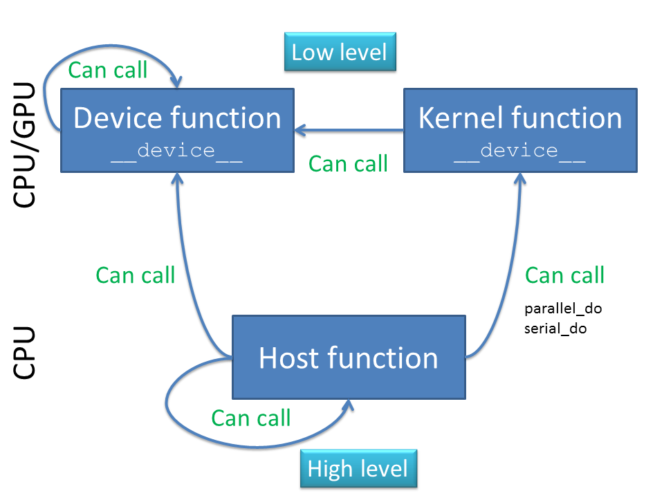
The following diagram illustrates the relationship between __kernel__, __device__ and host functions:
Summarized:
Both
__kernel__and__device__functions are low-level functions, they are natively compiled for CPU and/or GPU. This has the practical consequence that the functionality available for these functions is restricted. It is for example not possible toprint,loadorsaveinformation inside kernel or device functions.Host functions are high-level functions, typically they are interpreted (or Quasar EXE’s, compiled using the just-in-time compiler).
A kernel function is normally repeated for every element of a matrix. Kernel functions can only be called from host code (although in future support for CUDA 5.0 dynamic parallelism, this may change).
A device function can be called from host code, in which case it is normally interpreted (if not inlined), or from other device/kernel functions, in which case it is natively compiled.
The distinction between these three types of functions is necessary to allow GPU programming. Furthermore, it provides a mechanism (to some extent) to balance the work between CPU/GPU. As programmer, you know whether the code inside the function will be run on GPU/CPU. # Multi-level breaks in sequential loops
Sometimes, small language features can make a lot of difference (in terms of code readability, productivity etc.). In Quasar, multi-dimensional for-loops are quite common. Recently, I came across a missing feature for dealing with multi-dimensional loops.
Suppose we have a multi-dimensional for-loop, as in the following example:
for m=0..511
    for n=0..511
        im_out[m,n] = 255-im[m,n]
        if m==128
            break
        endif
        a = 4
    endfor
endfor
Suppose that we want to break outside the loop, as in the above code. This is useful for stopping the processing at a certain point. There is only one caveat: the break-statement only applies to the loop that surrounds it. In the above example, the processing of row 128 is simply stopped at column 0 (the loop over n is interrupted), but it is then resumed starting from row 129. Some programmers are not aware of this, sometimes this can lead to less efficient code, as in the following example:
for j = 0..size(V,0)-1
    for k=0..size(V,1)-1
        if V[j,k]
            found=[j,k]
            break
        endif
    endfor
endfor
Here we perform a sequential search, to find the first matrix element for which V[j,k] != 0. When this matrix element is found, the search is stopped. However, because the break statement stops the inner loop, the outer loop is still executed several times (potentially leading to a performance degradation).
1. Solution with extra variables
To make sure that we break outside the outer loop, we would have to introduce an extra variable:
break_outer = false
for j = 0..size(V,0)-1
    for k=0..size(V,1)-1
        if V[j,k]
            found=[j,k]
            break_outer = true
            break
        endif
    endfor
    if break_outer
        break
    endif
endfor
It is clear that this approach is not very readible. The additional variable break_outer is also a bit problematic (in the worst case, if the compiler can not filter it out, extra stack memory/registers will be required).
2. Encapsulation in a function
An obvious alternative is the use of a function:
function found = my_func()
    for j = 0..size(V,0)-1
        for k=0..size(V,1)-1
            if V[j,k]
                found=[j,k]
                break
            endif
        endfor
    endfor
endfunction
found = my_func()
However, the use of function is sometimes not desired for this case. It also involves extra work, such as adding the input/output parameters and adding a function call.
3. New solution: labeling loops
To avoid the above problems, it is now possible to label the for loops (as in e.g. ADA, java):
outer_loop:
    for j = 0..size(V,0)-1
    inner_loop:
        for k=0..size(V,1)-1
            if V[j,k]
                found=[j,k]
                break outer_loop
            endif
        endfor
    endfor
Providing labels to for-loops is optional, i.e. you only have to do it when it is needed. The new syntax is also supported by the following finding in programming literature: > In 1973 S. Rao Kosaraju refined the structured program theorem by proving that it’s possible to avoid adding additional variables in structured programming, as long as arbitrary-depth, multi-level breaks from loops are allowed. [11]
Note that Quasar has no goto labels (it will never have). The reasons are:
- Control flow blocks can always be used instead. Control flow blocks offer more visual cues which enhances the readability of the code.
- At the compiler-level, goto labels may make it more difficult to optimize certain operations (e.g. jumps to different scopes).
Remarks:
- This applies to the keyword
continueas well. - Labels can be applied to
for,repeat…untilandwhileloops. - In the future, more compiler functionality may be added to make use of the loop labels. For example, it may be possible to indicate that multiple loops (with the specified names) must be merged.
- It is not possible to break outside a parallel loop! The reason is that the execution of the different threads is (usually) non-deterministic, hence using breaks in parallel-loops would result in non-deterministic results.
- However, loop labels can be attached to either serial/parallel loops. A useful situation is an iterative algorithm with an inner/outer loop. # Placeholder ’_’ for functions with multiple return values
(feature originally suggested by Dirk Van Haerenborgh)
In Quasar, it is possible to define functions with multiple return values. An example is the sincos function which calculates the sine and the cosine of an angle simultaneously:
function [s, c] = sincos(theta)
    ...
endfunction
Sometimes, your function may return several values, such as an image and a corresponding weight matrix:
function [img, weight] = process(input_img)
    ...
endfunction
and it may happen that the weight image is in practice not needed on the caller side. Instead of introducing dummy variables, it is now possible to explicitly indicate that a return value is not needed (e.g. as in Python):
[img, _] = process(input_img)This way, the Quasar compiler is aware that it is not your intention to do something with the unused return value. In the future, it may even be possible that the output variable weight is optimized away (and not even calculated inside the function process).
In case you would - for some reason - forget to capture the return values, such as:
process(input_img)Then the compiler will generate a warning message, stating:
[Performance warning] Function ‘process’ returns 2 values that are ignored here. Please eliminate the return values in the function signature (when possible) or use the placeholder ‘[_,_]=process(.)’ to explicitly capture the unused return values.
In this case, it is recommended that you explicitly indicate the return values that are unused:
[_,_] = process(input_img)Variadic Functions and the Spread Operator
A new feature is the support for variadic functions in Quasar. Variadic functions are functions that can have a variable number of arguments. For example,
function [] = func(... args)
    for i=0..numel(args)-1
        print args[i]
    endfor
endfunction
func(1, 2, "hello")
Here, args is called a rest parameter (which is similar to ECMAScript 6). How does this work: when the function func is called, all arguments are packed in a cell vector which is passed to the function. Optionally, it is possible to specify the types of the arguments:
function [] = func(... args:vec[string])which indicates that every argument must be a string, so that the resulting cell vector is a vector of strings.
Several library functions in Quasar already support variadic arguments (e.g. print, plot, …), although now it is possible to define your own functions with variadic arguments.
Moreover, a function may have a set of fixed function parameters, optional function parameters and variadic parameters. The variadic parameters should always appear at the end of the function list (otherwise a compiler error will be generated)
function [] = func(a, b, opt1=1.0, opt2=2.0, ...args)
endfunction
This way, the caller of func can specify extra arguments when desired. This allows adding extra options for e.g., solvers.
Variadic device functions
It is also possible to define device functions supporting variadic arguments. These functions will be translated by the back-end compilers to use cell vectors with dynamically allocated memory (it is useful to consider that this may have a small performance cost).
An example:
function sum = __device__ mysum(... args:vec)
    sum = 0.0
    for i=0..numel(args)-1
        sum += args[i]
    endfor
endfunction

function [] = __kernel__ mykernel(y : vec, pos : int)
    y[pos]= mysum(11.0, 2.0, 3.0, 4.0)
endfunction
Note that variadic kernel functions are currently not supported.
Variadic function types
Variadic function types can be specified as follows:
fn : [(...??) -> ()]
fn2 : [(scalar, ...vec[scalar]) -> ()]
This way, functions can be declared that expect variadic functions:
function [] = helper(custom_print : [(...??) -> ()])
    custom_print("Stage", 1)
    ...
    custom_print("Stage", 2)
endfunction

function [] = myprint(...args)
    for i=0..numel(args)-1
        fprintf(f, "%s", args[i])
    endfor
endfunction

helper(myprint)
The spread operator
Unpacking vectors The spread operator unpacks one-dimensional vectors, allowing them to be used as function arguments or array indexers. For example:
pos = [1, 2]
x = im[...pos, 0]
In the last line, the vector pos is unpacked to [pos[0], pos[1]], so that the last line is in fact equivalent with
x = im[pos[0], pos[1], 0]Note that the spread syntax ... makes the writing of the indexing operation a lot more convenient. An additional advantage is that the spread operator can be used, without knowing the length of the vector pos. Assume that you have a kernel function in which the dimension is not specified:
function [] = __kernel__ colortransform (X, Y, pos)
    Y[...pos, 0..2] = RGB2YUV(Y[...pos, 0..2])
endfunction
This way, the colortransform can be applied to a 2D RGB image, as well as a 3D RGB image.
Similarly, if you have a function taking three arguments, such as:
luminance = (R,G,B) -> 0.2126 * R + 0.7152 * G + 0.0722 * BThen, typically, to pass an RGB vector c to the function luminance, you would use:
c = [128, 42, 96]
luminance(c[0],c[1],c[2])
Using the spread operator, this can simply be done as follows:
luminance(...c) Passing variadic arguments The spread operator also has a role when passing arguments to functions.
Consider the following function which returns two output values:
function [a,b] = swap(A,B)
    [a,b] = [B,A]
endfunction
And we wish to pass both output values to one function
function [] = process(a, b)
    ...
endfunction
Then using the spread operator, this can be done in one line:
process(...swap(A,B))Here, the multiple values [a,b] are unpacked before they are passed to the function process. This feature is particularly useful in combination with variadic functions.
Notes:
Only vectors (i.e., with dimension 1) can currently be unpacked using the spread operator. This may change in the future.
Within kernel/device functions, the spread operator is currently supported on fixed-length vectors
vecX,cvecX,ivecX(this means: the compiler should be able to determine the length of the vector statically).Within host functions, cell vectors can be unpacked as well
The spread operator can be used for concatenating vectors and scalars:
  a = [1,2,3,4]
  b = [6,7,8]
  c = [...a, 4, ...b]
where
cwill be a vector of length 8. For small vectors, this is certainly a good approach. For long vectors, this technique may have a poor performance, due to the concatenation being performed on the CPU. In the future, the automatic kernel generator may be extended, to generate efficient kernel functions for the concatenation.
Variadic output parameters
The output parameter list does not support the variadic syntax .... Instead, it is possible to return a cell vector of a variable length.
function [args] = func_returning_variadicargs()
    args = vec[??](10)
    args[0] = ...
endfunction
The resulting values can then be captured in the standard way as output parameters:
a = func_returning_variadicargs() % Captures the cell vector
[a] = func_variadicargs() % Captures the first element, and generates an
                          % error if more than one element is returned
[a, b] = func_variadicargs() % Captures the first and second elements and
                             % generates an error if more than one element
                             % is returned
Additionally, using the spread operator, the output parameter list can be unpacked and passed to any function:
myprint(...func_variadicargs())The main function revisited
The main function of a Quasar program can be variadic, i.e. accepting a variable number of parameters.
function [] = main(...args)or
function [] = main(...args : vec[??])This way, parameters can be passed through the command-line:
Quasar.exe myprog.q 1 2 3 "string"There are in fact 4 possibilities:
main functions with fixed parameters
function [] = main(a, b)In this case, the user is required to specify the values for the parameters
main functions with fixed and/or optional parameters
function [] = main(a=0.0, b=0.5)This way, the programmer can specify a default value for the parameters
main functions with fixed/optional/variadic parameters
function [] = main(fixed, a=0.0, b=0.5, ...args)Using this approach, some of the parameters are mandatory, other parameters are optional. Additionally it is possible to pass extra values to the main function, which the program will process. # Construction of cell matrices
In Quasar, it is possible to construct cell vectors/matrices, similar to in MATLAB:
A = {1,2,3j,zeros(4,4)}Note: the old-fashioned alternative was to construct cell matrices using the function cell, or vec[vec], vec[mat], vec[cube], … For example:
A = cell(4)
A[0] = 1j
A[1] = 2j
A[2] = 3j
A[3] = 4j
Note that this notation is not very elegant, compared to A={1j,2j,3j,4j}. Also it does not allow the compiler to fully determine the type of A (the compiler will find type(A) == "vec[??]" rather than type(A) == "cvec"). In the following section, we will discuss the type inference in more detail.
Type inference
Another new feature of the compiler is that it attempts to infer the type from cell matrices. In earlier versions, all cell matrices defined with the above syntax, had type vec[??]. Now, this has changed, as illustrated by the following example:
    a = {[1, 2],[1, 2, 3]}
    print type(a)            % Prints vec[vec[int]]

    b = {(x->2*x), (x->3*x), (x->4*x)}
    print type(b)            % Prints [ [??->??] ]

    c = {{[1, 2],[1,2]},{[1, 2, 3],[4, 5, 6]}}
    print type(c)            % Prints vec[vec[vec[int]]]

    d = { [ [2, 1], [1, 2] ], [ [4, 3], [3, 4] ]}
    print type(d)            % Prints vec[mat]

    e = {(x:int->2*x), (x:int->3*x), (x:int->4*x)}
    print type(e)            % Prints vec[ [int->int] ]
This allows cell matrices that are constructed with the above syntax to be used from kernel functions. A simple example:
    d = {eye(4), ones(4,4)}

    parallel_do(size(d[0]), d,
        __kernel__ (d : vec[mat], pos : ivec2) -> d[0][pos] += d[1][pos])
    print d[0]
The output is:
       [ [2,1,1,1],
         [1,2,1,1],
         [1,1,2,1],
         [1,1,1,2] ]
Boundary access modes in Quasar (see #23)
In earlier versions of Quasar, the boundary extension modes (such as 'mirror, 'circular) only affected the __kernel__ and __device__ functions.
To improve transparency, this is has recently changed. This has the consequence that the following get access modes needed to be supported by the runtime:
(no modifier)     % =error (default) or zero extension (kernel, device function)
safe              % zero extension
mirror            % mirroring near the boundaries
circular          % circular boundary extension
clamped           % keep boundary values
unchecked         % results undefined when reading outside
checked           % error when reading outside
Implementation details: there is a bit of work involved, because it needs to be done for all data types (int8, int16, int32, uint8, uint16, uint32, single, double, UDT, object, …), for different dimensions (vec, mat, cube), and for both matrix getters / slice accessors. perhaps the reason that you will not see this feature implemented in other programming languages: 5 x 10 x 3 x 2 = 300 combinations (=functions to be written). Luckily the use of generics in C# alleviates the problem, reducing it (after a bit of research) to 6 combinations (!) where each algorithm has 3 generic parameters. Idem for CUDA computation engine.
Note that the modifier unchecked should be used with care: only when you are 100% sure that the function is working properly and that there are no memory accesses outside the matrix. A good approach is to use checked first, and when you find out that there never occur any errors, you can switch to unchecked, in other to gain a little speed-up (typically 20%-30% on memory accesses).
Now I would like to point out that the access modifiers are not part of type of the object itself, as the following example illustrates:
A : mat'circular = ones(10, 10)
B = A    % boundary access mode: B : mat'circular
C : mat'unchecked = A
Here, both B and C will hold a reference to the matrix A. However, B will copy the access modifier from A (through type inference) and C will override the access modifier of A. The result is that the access modifiers for A, B and C are circular, circular and unchecked, respectively. Even though there is only one matrix involved, there are effectively two ways of accessing the data in this matrix.
Now, to make things even more complicated, there are also put access modes. But for implementation complexity reasons (and more importantly, to avoid unforeseen data races in parallel algorithms), the number of options have been reduced to three:
safe (default)      % ignore writing outside the boundaries
unchecked           % writing outside the boundaries = crash!
checked             % error when writing outside the boundaries
This means that 'circular, 'mirror, and 'clamped are mapped to 'safe when writing values to the matrix. For example:
A : vec'circular = [1, 2, 3]
A[-1] = 0   % Value neglected
The advantage will then be that you can write code such as:
A : mat'circular = imread("lena_big.tif")[:,:,1]
B = zeros(size(A))
B[-127..128,-127..128] = A[-127..128,-127..128]
Boundary Access Testing through High Level Inference
To avoid vector/matrix boundary checks, the modifier 'unchecked can be used. This often gives a moderate performance benefit, especially when used extensively inside kernel functions.
The use of 'unchecked requires the programmer to know that the index boundaries will not be exceeded (e.g., after extensive testing with the default, 'checked). To avoid “Segment violations” causing the Redshift GUI to crash, Quasar has a setting “Out of bounds checks” that will internally override the 'unchecked modifiers and convert all these modifiers to 'checked. However, with this technique, the performance benefit of 'unchecked is lost unless the programmer switches off the “Out of bounds checks”.
Solution: compile-time high level inference
As a better solution, the compiler will now infer from the context several cases in which the boundary checks can be dropped. Consider the following use-case:
im  = imread("lena_big.tif")[:,:,1]
im_out = zeros(size(im))

for m=0..size(im,0)-1
    for n=0..size(im,1)-1
        im_out[m,n] = 4*im[m,n]
    endfor
endfor
In this case, the Quasar compiler knows that the entire image is traversed with the double loop (checking the dimensions size(im,0), size(im,1)). Moreover, because im_out = zeros(size(im)), the compiler internally assumes that size(im_out) == size(im). This way, the compiler can decide that the boundary accesses im_out[m,n] and im[m,n] are all safe and can be dropped! Even when the option “Out of bounds checks” is turned on!
This way, existing Quasar programs can benefit from performance improvements without any further change. In some cases, the programmer can help the compiler by making assertions on the matrix dimensions. For example:
function [] = process(im : mat, im_out : mat)
    assert(size(im) == size(im_out))
    for m=0..size(im,0)-1
        for n=0..size(im,1)-1
            im_out[m,n] = 4*im[m,n]
        endfor
    endfor
endfunction
What basically happens, is that the boundary checks are moved outside the loop: the assertion will check the dimensions of im_out and assure that the two-dimensional loop is safe! The assertion check outside the loop is much faster than boundary checks for every position inside the loop.
Currently, the inference possibilities of the compiler are limited to simple (but often occurring) use-cases. In the future, there will be more cases that the compiler can recognize. # Dynamic Memory Allocation on CPU/GPU
In some algorithms, it is desirable to dynamically allocate memory inside __kernel__ or __device__ functions, for example:
When the algorithm processes blocks of data for which the maximum size is not known in advance.
When the amount of memory that an individual thread uses is too large to fit in the shared memory or in the registers. The shared memory of the GPU consists of typically 32K, that has to be shared between all threads in one block. For single-precision floating point vectors
vecor matricesmatand for 1024 threads per block, the maximum amount of shared memory is 32K/(1024*4) = 8 elements. The size of the register memory is also of the same order: 32 K for CUDA compute architecture 2.0.
Example: brute-force median filter
So, suppose that we want to calculate a brute-force median filter for an image (note that there exist much more efficient algorithms based on image histograms, see immedfilt.q). The filter could be implemented as follows:
we extract a local window per pixel in the image (for example of size
13x13).the local window is then passed to a generic median function, that sorts the intensities in the local window and returns the median.
The problem is that there may not be enough register memory for holding a local window of this size. 1024 threads x 13 x 13 x 4 = 692K!
The solution is then to use a new Quasar runtime & compiler feature: dynamic kernel memory. In practice, this is actually very simple: first ensure that the compiler setting “kernel dynamic memory support” is enabled. Second, matrices can then be allocated through the regular matrix functions zeros, complex(zeros(.)), uninit, ones.
For the median filter, the implementation could be as follows:
% Function: median
% Computes the median of an array of numbers
function y = __device__ median(x : vec)
    % to be completed
endfunction

% Function: immedfilt_kernel
% Naive implementation of a median filter on images
function y = __kernel__ immedfilt_kernel(x : mat, y : mat, W : int, pos : ivec2)

    % Allocate dynamic memory (note that the size depends on W,
    % which is a parameter for this function)
    r = zeros((W*2)^2)

    for m=-W..W-1
        for n=-W..W-1
            r[(W+m)*(2*W)+W+n] = x[pos+[m,n]]
        endfor
    endfor

    % Compute the median of the elements in the vector r
    y[pos] = median(r)
endfunction
For W=4 this algorithm is illustrated in the figure below:
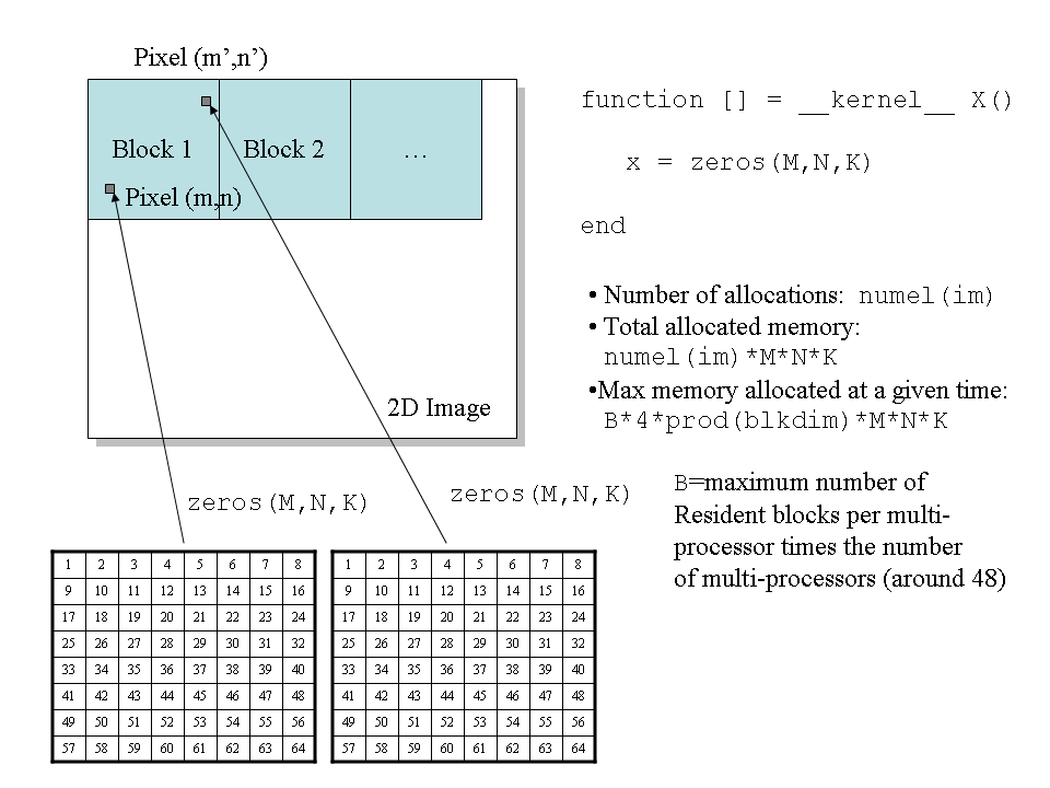 Figure 1. dynamic memory allocation inside a kernel function.
Parallel memory allocation algorithm
To support dynamic memory, a special parallel memory allocator was designed. The allocator has the following properties:
The allocation/disposal is distributed in space and does not use lists/free-lists of any sort.
The allocation algorithm is designed for speed and correctness.
To accomplish such a design, a number of limitations were needed:
The minimal memory block that can be allocated is 1024 bytes. If the block size is smaller then the size is rounded up to 1024 bytes.
When you try to allocate a block with size that is not a pow-2 multiple of 1024 bytes (i.e.
1024*2^NwithNinteger), then the size is rounded up to a pow-2 multiple of 1024 bytes.The maximal memory block that can be allocated is 32768 bytes (=2^15 bytes). Taking into account that this can be done per pixel in an image, this is actually quite a lot!
The total amount of memory that can be allocated from inside a kernel function is also limited (typically 16 MB). This restriction is mainly to ensure program correctness and to keep memory free for other processes in the system.
It is possible to compute an upper bound for the amount of memory that will be allocated at a given point in time. Suppose that we have a kernel function, that allocates a cube of size M*N*K, then:
max_memory = NUM_MULTIPROC * MAX_RESIDENT_BLOCKS * prod(blkdim) * 4*M*N*KWhere prod(blkdim) is the number of elements in one block, MAX_RESIDENT_BLOCKS is the maximal number of resident blocks per multi-processor and NUM_MULTIPROC is the number of multiprocessors.
So, suppose that we allocate a matrix of size 8x8 on a Geforce 660Ti then:
max_memory = 5 * 16 * 512 * 4 * 8 * 8 = 10.4 MBThis is still much smaller than what would be needed if one would consider pre-allocation (in this case this number would depend on the image dimensions!)
Comparison to CUDA malloc
CUDA has built-in malloc(.) and free(.) functions that can be called from device/kernel functions, however after a few performance tests and seeing warnings on CUDA forums, I decided not to use them. This is the result of a comparison between the Quasar dynamic memory allocation algorithm and that of NVidia:
    Granularity: 1024
    Memory size: 33554432
    Maximum block size: 32768
    Start - test routine

    Operation took 183.832443 msec [Quasar]
    Operation took 1471.210693 msec [CUDA malloc]
    Success
I obtained similar results for other tests. As you can see, the memory allocation is about 8 times faster using the new apporach than with the NVidia allocator.
Why better avoiding dynamic memory
Even though the memory allocation is quite fast, to obtain the best performance, it is better to avoid dynamic memory:
The main issue is that kernel functions using dynamic memory also require several read/write accesses to the global memory. Because dynamically allocated memory has typically the size of hundreds of KBs, the data will not fit into the cache (of size 16KB to 48KB). Correspondingly: the cost of using dynamic memory is in the associated global memory accesses!
Please note that the compiler-level handling of dynamic memory is currently in development. As long as the memory is “consumed” locally as in the above example, i.e. not written to external data structures the should not be a problem.
CUDA - Device Functions Across Modules
Device functions are useful to implement common CPU and GPU routines once in order to later use them from different other kernel or device functions (also see the function overview).
An example is the sinc function in system.q:
sinc = __device__ (x : scalar) -> (x == 0.0) ? 1.0 : sin(pi*x)/(pi*x)By this definition, the sinc function can be used on scalar numbers from both host functions as kernel/device functions.
However, when a device function is defined in one module and used in an another module, there is one problem for the CUDA engine. The compiler will give the following error:
Cannot currently access device function 'sinc' defined in
'system.q' from 'foo.q'. The reason is that CUDA 4.2 does not
support static linking so device functions must be defined in the
same compilation unit.
By default, __device__ functions are statically linked (in C/C++ linker terminology). However, CUDA modules are standalone, which makes it impossible to refer from device functions in one module to another module.
There are however two work-arounds:
the first work-around is to define the function using a lambda expression, by making sure that function inlining is enabled (the compiler setting
COMPILER_LAMBDAEXPRESSION_INLININGshould have valueOnlySuitableorAlways).This way, the function will be expanded inline by the Quasar compiler and the problem is avoided.
the second work-around is to use function pointers to prevent static linking. Obviously, this has an impact on performance, therefore the compiler setting
COMPILER_USEFUNCTIONPOINTERSneeds to be set toAlways(default value =SmartlyAvoid).
If possible, try to define the functions in such a way that device functions are only referred to from the module in which they are defined. If this is not possible/preferred, use work-around #1 (i.e. define the function as a lambda expression and enable automatic function inlining). # CUDA Synchronization on Global Memory
Because the amount of shared memory is limited (typically 32K), one may think that straightforward extension is to use the global memory for inter-thread communication, because the global memory does not have this size restriction (typically it is 1-2GB or more). This would then give a small performance loss compared to shared memory, but the benefit of caching and sharing data between threads could make this option attractive for certain applications.
However, this may be a bit more trickier than expected: in practice, this turns out not to work at all!
Consider for example the following kernel, that performs a 3x3 mean filter where the shared memory has been replaced by global memory (tmp):
tmp = zeros(64,64,3)

function [] = __kernel__ kernel(x : cube, y : cube, pos : vec3, blkpos : vec3, blkdim : vec3)

    tmp[blkpos] = x[pos]

    if blkpos[0] < 2
        tmp[blkpos+[blkdim[0],0,0]] = x[pos+[blkdim[0],0,0]]
    endif

    if blkpos[1] < 2
        tmp[blkpos+[0,blkdim[1],0]] = x[pos+[0,blkdim[1],0]]
    endif

    if blkpos[0] < 2 && blkpos[1] < 2
        tmp[blkpos+[blkdim[0],blkdim[1],0]] = x[pos+[blkdim[0],blkdim[1],0]]
    endif

    syncthreads

    y[pos] = (tmp[blkpos+[0,0,0]] +
              tmp[blkpos+[0,1,0]] +
              tmp[blkpos+[0,2,0]] +
              tmp[blkpos+[1,0,0]] +
              tmp[blkpos+[1,1,0]] +
              tmp[blkpos+[1,2,0]] +
              tmp[blkpos+[2,0,0]] +
              tmp[blkpos+[2,1,0]] +
              tmp[blkpos+[2,2,0]]) * (1/9)
endfunction

im = imread("lena_big.tif")
im_out = zeros(size(im))

parallel_do(size(im_out),im,im_out,kernel)
Figure 1. Using shared memory: the expected outcome of a 3x3 average filter.

Figure 2. Using global memory: not what one would expect!
Although the algorithm works correctly with shared memory, for global memory the output is highly distorted. What is going on here?
The assumption that is made in case of shared memory, is that the blocks are processed by the GPU completely independently from each other.
However, for obvious performance reasons, this is not the case, and the GPU starts already block #2 while finishing block #1.
Shared memory is a special case, because shared memory actually resides on the multiprocessors, and a thread can only access the shared memory from the multiprocessor that it is running on.
The solution would then be to do to make the global memory access block-dependent. However, doing so would be very architecture-dependent and not portable. So this is not recommended. # CUDA - Dealing with low kernel occupancy issues
I recently discovered an issue that led the runtime to execute a kernel at a low occupancy (NVidia explanation). The problem was quite simple: the multiplication of a (3xN) matrix with an (Nx3) matrix, where N is very large, e.g. 2^18 (resulting in a 3x3 matrix).
The runtime currently uses the simplest possible algorithm for multiplication, using a block of size 3x3. However, the occupancy in this case is approx. 9/MAX_THREADS, which is about 3.33% in my case. This means that the performance of this simple operation is (theoretically) decreased by up to a factor 30! Only 9 threads are spawn, while the hardware can support up to 1024. (Note: in the latest versions of Quasar Redshift, the occupancy can be viewed in the profiler).
For this reason, I wrote a Quasar program to use a larger block size. The program also uses shared memory with the parallel sum reduction, so even the quite simple matrix multiplication results in an advanced implementation:-)
This program will be integrated in the runtime, so in the future, the user does not have to worry about this anymore. Nevertheless, it can be good to know how certain operations are implemented efficiently internally.
function y = matrix_multiply(a, b)

    [M,N] = [size(a,0),size(b,1)]
    y = zeros(M,N)

    function [] = __kernel__ kernel(a : mat'unchecked, b : mat'unchecked, blkdim : ivec3, blkpos : ivec3)

        n = size(a,1)
        bins = shared(blkdim)
        nblocks = int(ceil(n/blkdim[0]))

        % step 1 - parallel sum
        val = 0.0
        for m=0..nblocks-1
            if blkpos[0] + m*blkdim[0] < n
            c = blkpos[0] + m*blkdim[0]
            val += a[blkpos[1],c] * b[c,blkpos[2]]
            endif
        endfor
        bins[blkpos] = val

        % step 2 - reduction
        syncthreads
        bit = 1
        while bit < blkdim[0]
            if mod(blkpos[0],bit*2) == 0
            bins[blkpos] += bins[blkpos + [bit,0,0]]
            endif
            syncthreads
            bit *= 2
        endwhile

        % write output
        if blkpos[0] == 0
            y[blkpos[1],blkpos[2]] = bins[0,blkpos[1],blkpos[2]]
        endif
    endfunction

    P = prevpow2(max_block_size(kernel,[size(a,1),M*N])[0])
    parallel_do([P,M,N],a,b,kernel)
endfunction

function [] = main()
    im = imread("lena_big.tif")

    n = prod(size(im,0..1))
    x = reshape(im,[n,3])

    tic()
    for k=0..99
    y1 = transpose(x)*x
    endfor
    toc()  % 3.5 seconds

    tic()
    for k=0..99
    y2 = matrix_multiply(transpose(x),x)
    endfor
    toc()  % 1.3 seconds

    print y1
    print y2
endfunction
CUDA - Memory manager enhancements I (advanced)
There are some problems operating on large images that do not fit into the GPU memory. The solution is to provide a FAULT-TOLERANT mode, in which the operations are completely performed on the CPU (we assume that the CPU has more memory than the GPU). Of course, running on the CPU comes at a performance hit. Therefore I will add some new configurable settings in this enhancement.
Please note that GPU memory problems can only occur when the total amount of memory used by one single kernel function > (max GPU memory - reserved mem) * (1 - fragmented mem%). For a GPU with 1 GB, this might be around 600 MB. Quasar automatically transfers memory buffers back to the CPU memory when it is running out of GPU space. Nevertheless, this may not be sufficient, as some very large images can take all the space of the GPU memory (for example 3D datasets).
Therefore, three configurable settings are added to the runtime system (Quasar.Redshift.config.xml):
RUNTIME_GPU_MEMORYMODELwith possible values:
- SmallFootPrint - A small memory footprint - opts for conservative memory allocation leaving a lot of GPU memory available for other programs in the system
- MediumFootprint (*) - A medium memory footprint - the default mode
- LargeFootprint - chooses aggressive memory allocation, consuming most of the available GPU memory quickly, and leaving no memory available for other applications. This option is recommended for GPU memory intensive applications.
RUNTIME_GPU_SCHEDULINGMODEwith possible values:
- MaximizePerformance - Attempts to perform as many operations as possible on the GPU (potentially leading to memory failure if there is not sufficient memory available. Recommended for systems with a lot of GPU memory).
- MaximizeStability (*) - Performs operations on the CPU if there is not GPU memory available. For example, processing 512 MB images when the GPU only has 1 GB memory available. The resulting program may be slower. (FAULT-TOLERANT mode)
RUNTIME_GPU_RESERVEDMEM
- The amount of GPU memory reserved for the system (in MB) and/or other processes. The Quasar runtime system will not use the reserved memory (so that other desktop programs can still run correctly). Default value = 160 MB. This value can be decreased at the user’s risk to obtain more GPU memory for processing (desktop applications such as Firefox may complain…)
Please note that the “imshow” function also makes use of the reserved system GPU memory (the CUDA data is copied to an OpenGL texture).
(*) default
CUDA Error handling
For the Quasar run-time, the CUDA error handling mechanism is quite tricky, in the sense that when an error occurs, the GPU device often has to be reinitialized. Consequently, at this time, all data stored in the GPU memory is lost.
The following article gives a more detailed overview of CUDA’s error handling mechanism. http://www.drdobbs.com/parallel/cuda-supercomputing-for-the-masses-part/207603131.
Some considerations:
- “A human-readable description of the error can be obtained from”:
char *cudaGetErrorString(cudaError_t code);In practice, this function will return useless “Unknown error”, “Invalid context”, “Kernel execution failed”
“CUDA also provides a method, cudaGetLastError, which reports the last error for any previous runtime call in the host thread. This has multiple implications: the asynchronous nature of the kernel launches precludes explicitly checking for errors with cudaGetLastError.” => This simply means that error handling does not work in asynchronous mode (concurrent kernel execution).
“When multiple errors occur between calls to cudaGetLastError, only the last error will be reported. This means the programmer must take care to tie the error to the runtime call that generated the error or risk making an incorrect error report to users” => There is no way to find if any other error is raised previously, or which component caused which error.
Practically, when CUDA returns an error, the Quasar runtime attempts to guess what is going on. This can be particularly daunting, especially when concurrent kernel execution is enabled (the flame icon in Redshift).
However, since CUDA 5.5, a stream callback mechanism was introduced and since recently, Quasar is able to use this mechanism for concurrent kernels, even when multiple kernels are launched in sequence. This allows correct handling of errors raised in kernel function, such as:
- matrix out of boundary access (
'checkedmode) - a call to the function
error - an assertion failure
assert(false) - an integer overflow
- NaN or Inf (when checking enabled)
- out of shared memory
- out of dynamic memory
- CUDA unknown error
Users working with CUDA 4.2 (or earlier) should either 1) turn off the concurrent kernel execution or 2) upgrade to CUDA 5.5.
Quasar - slow shared memory, why?
Sometimes, when you use shared memory in Quasar programs, you may notice that using shared memory is significantly slower than directly accessing the global memory, which is very counterintuitive.
The reason is simple: by default, Quasar performs boundary checks at runtime, even inside the kernel functions. This is to ensure that all your kernels are programmed correctly and to catch otherwise undetectable errors very early.
Instead of using the default access:
xr = shared(M,N)it may be useful to disable the boundary checks for the variable:
xr : mat'unchecked = shared(M,N)Note that boundary checking is an option that can be enabled/disabled in the program settings dialog box, or alternatively by editing Quasar.Redshift.config.xml:
  <setting name="COMPILER_OUTOFBOUNDS_CHECKS">
    <value>False</value>
  </setting>
Finally, see also this trick that allows you to further optimize kernel functions that use shared memory. # CUDA: Specifying shared memory bounds
In this Section, a technique is described to use the shared memory of the GPU in a more optimal way, through specification of the amount of memory that a kernel function will actually use.
The maximum amount of shared memory that Quasar kernel functions can currently use is 32K (32768 bytes). Actually, the maximum amount of shared memory of the device is 48K (16K is reserved for internal purposes). The GPU may process several blocks at the same time, however there is one important restriction:
The total number of blocks that can be processed at the same time also depends on the amount of shared memory that is used by each block.
For example, if one block uses 32K, then it is not possible to launch a second block at the same time, because 2 x 32K > 48K. In practice, your kernel function may only use e.g. 4K instead of 32K. This would then allow 48K/4K = 12 blocks to be processed at the same time.
Originally, the Quasar compiler either reserved 0K or 32K shared memory per block, depending on whether the kernel function allocated shared memory. Shared memory is dynamically allocated from within the kernel function. This actually deteriorates the performance, because N*32K < 48K requires N=1. So there is only one block that can be launched simultaneously.
In the latest version, the compiler is able to infer the total amount of shared memory that is being used through the proportional logic system. For example, if you request:
x = shared(20,3,6)the compiler will reserve 20 x 3 x 6 x 4 bytes = 1440 bytes for the kernel function. Often the arguments of the function shared are non-constant. In this case you can use assertions.
assert(M<8 && N<20 && K<4)
x = shared(M,N,K)
Due to the above assertion, the compiler is able to infer the amount of required shared memory. In this case: 8 x 20 x 4 x 4 bytes = 2560 bytes. The compiler then gives the following message:
Information: shared_mem_test.q - line 17: Calculated an upper bound for
the amount of shared memory: 2560 bytes
The assertion also allows the runtime system to check whether not too much shared memory will be allocated. In case N would exceed 20, the runtime system will give an error message.
Note: the compiler does not recognize yet all possible assertions that restrict the amount of shared memory. For example assert(numel(blkdim)<=1024); x = shared(blkdim) will not work yet. In the future, more use cases like this will be accepted.
Conclusion:
When implementing a kernel function that uses shared memory, it is recommended to give hints to the compiler about the amount of shared memory that the function will actually use. This can be done using assertions.
The best is to keep the amount of memory used by a kernel function as low as possible. This allows multiple blocks to be processed in parallel. # Assert the Truth, Unassert the Untruth
Quasar has a logic system, that is centered around the assert function and that can be useful for several reasons:
Assertions can be used for testing a specified condition, resulting in a runtime error (
error) if the condition is not met:assert(positiveNumber>0,"positiveNumber became negative while it shouldn't")Assertions can also help the optimization system. For example, the type of variables can be “asserted” using type assertions:
assert(type(cubicle, "cube[cube]"))The compiler can then verify the type of the variable
cubicleand if it is not known at this stage, knowledge can be inserted into the compiler, resulting in the compilation message:assert.q - Line 4: [info] 'cubicle' is now assumed to be of type 'cube[cube]'.At runtime, the assert function just behaves like usual, resulting in an error if the condition is not met.
Assertions are useful in combination with reduction-where clauses:
reduction (x : scalar) -> abs(x) = x where x >= 0If we previously assert that
xis a positive number, then this assertion will eliminate the runtime check forx >= 0.Assertions can be used to cut branches:
  assert(x > 0 && x < 1)
  if x < 0
      ...
  endif
Here, the compiler will determine that the
if-block will never be executed, so it will destroy the entire content of theif-block, resulting in a compilation message:assert.q - Line 10: [info] if-branch is cut due to the assertions `x > 0 && x < 1`.Similarly, pre-processor branches can be constructed with this approach.
Assertions can be combined with generic function specialization. Later more about this.
It is not possible to fool the compiler. For example, if the compiler can determine at compile-time that the assertion will never be met, an error will be generated, and it will not be even possible to run the program.
Logic system
The Quasar compiler has now a propositional logic system, that is able to “reason” about previous assertions. Also, different assertions can be combined using the logical operators AND &&, OR || and NOT !.
There are three meta functions that help with assertions:
$check(proposition)checks whetherpropositioncan be satisfied, given the previous set of assertions, resulting in three possible values:"Valid","Satisfiable"or"Unsatisfiable".$assump(variable)lists all assertions that are currently known about a variable, including the implicit type predicates that are obtained through type inference. Note that the result of$assumpis an expression, so for visualization it may be necessary to convert it to a textual representation using$str(.)(to avoid the expression from being evaluated).$simplify(expr)simplifies logic expressions based on the knowledge that is inserted through assertions.
Types of assertions
There are different types of assertions that can be combined in a transparent way.
Equalities
The most simple cases of assertions are the equality assertions a==b. For example:
symbolic a, b
assert(a==4 && b==6)

assert($check(a==5)=="Unsatisfiable")
assert($check(a==4)=="Valid")
assert($check(a!=4)=="Unsatisfiable")
assert($check(b==6)=="Valid")
assert($check(b==3)=="Unsatisfiable")
assert($check(b!=6)=="Unsatisfiable")
assert($check(a==4 && b==6)=="Valid")
assert($check(a==4 && b==5)=="Unsatisfiable")
assert($check(a==4 && b!=6)=="Unsatisfiable")
assert($check(a==4 || b==6)=="Valid")
assert($check(a==4 || b==7)=="Valid")
assert($check(a==3 || b==6)=="Valid")
assert($check(a==3 || b==5)=="Unsatisfiable")
assert($check(a!=4 || b==6)=="Valid")

print $str($assump(a)),",",$str($assump(b)) % prints (a==4),(b==6)
Here, we use symbolic to declare symbolic variables (variables that are not to be “evaluated”, i.e. translated into their actual value since they don’t have a specific value). Next, the function assert is used to test whether the $check(.) function works correctly (=self-checking).
Inequalities
The propositional logic system can also work with inequalities:
symbolic a
assert(a>2 && a<4)
assert($check(a>1)=="Valid")
assert($check(a>3)=="Satisfiable")
assert($check(a<3)=="Satisfiable")
assert($check(a<2)=="Unsatisfiable")
assert($check(a>4)=="Unsatisfiable")
assert($check(a<=2)=="Unsatisfiable")
assert($check(a>=2)=="Valid")
assert($check(a<=3)=="Satisfiable")
assert($check(!(a>3))=="Satisfiable")
Type assertions
As in the above example:
assert(type(cubicle, "cube[cube]"))Please note that assertions should not be used with the intention of variable type declaration. To declare the type of certain variables there is a more straightforward approach:
cubicle : cube[cube]Type assertions can be used in functions that accept generic ?? arguments, then for example to ensure that a cube[cube] is passed depending on another parameter.
User-defined properties of variables
It is also possible to define “properties” of variables, using a symbolic declaration. For example:
symbolic is_a_hero, Jan_AeltermanThen you can assert:
assert(is_a_hero(Jan_Aelterman))Correspondingly, if you perform the test:
print $check(is_a_hero(Jan_Aelterman))   % Prints: Valid
print $check(!is_a_hero(Jan_Aelterman))  % Prints: Unsatisfiable
If you then try to assert the opposite:
assert(!is_a_hero(Jan_Aelterman))The compiler will complain:
assert.q - Line 119: NO NO NO I don't believe this, can't be true!
Assertion '!(is_a_hero(Jan_Aelterman))' is contradictory with 'is_a_hero(Jan_Aelterman)'
Unassert
In some cases, it is neccesary to undo certain assertions that were previously made. For this task, the function unassert can be used:
unassert(propositions)This function only has a meaning at compile-time; at run-time nothing needs to be done.
For example, if you wish to reconsider the assertion is_a_hero(Jan_Aelterman) you can write:
unassert(is_a_hero(Jan_Aelterman))

print $check(is_a_hero(Jan_Aelterman))   % Prints: most likely not
print $check(!is_a_hero(Jan_Aelterman))  % Prints: very likely
Alternatively you could have written:
unassert(!is_a_hero(Jan_Aelterman))

print $check(is_a_hero(Jan_Aelterman))   % Prints: Valid
print $check(!is_a_hero(Jan_Aelterman))  % Prints: Unsatisfiable
Reductions with where-clauses
Recently, reduction where-clauses have been implemented. The where clause is a condition that determines at runtime (or at compile time) whether a given reduction may be applied. There are two main use cases for where clauses:
- To avoid invalid results: In some circumstances, applying certain reductions may lead to invalid results (for example a real-valued sqrt function applied to a complex-valued input, derivative of tan(x) in pi/2…)
- For optimization purposes.
For example:
reduction (x : scalar) -> abs(x) = x where x >= 0
reduction (x : scalar) -> abs(x) = -x where x < 0
In case the compiler has no information on the sign of x, the following mapping is applied:
abs(x) -> x >= 0 ? x : (x < 0 ? -x : abs(x))And the evaluation of the where clauses of the reduction is performed at runtime. However, when the compiler has information on x (e.g. assert(x <= -1)), the mapping will be much simpler:
abs(x) -> -xNote that the abs(.) function is a trivial example, in practice this could be more complicated:
reduction (x : scalar) -> some_op(x, a) = superfast_op(x, a) where 0 <= a && a < 1
reduction (x : scalar) -> some_op(x, a) = accurate_op(x, a) where 1 <= a
Meta (or macro) functions
Note: this section gives more advanced info about how internal routines of the compiler can be accessed from user code.
Quasar has a special set of built-in functions, that are aimed at manipulating expressions at compile-time (although in the future the implementation may also allow them to be used at run-time). The functions are special, because actually, they do not follow the regular evaluation order (i.e. they can be evaluated from the outside to the inside of the expression, depending on the context). To make the difference clear with the regular functions, these functions start with prefix $.
For example, x is an expression, as well as x+2 or (x+y)*(3*x)^99. A string can be converted (at runtime) to an expression using the function eval. This is useful for runtime processing of expressions for example entered by the user. However, the opposite is also possible:
print $str((x+y)*(3*x)^99)
% Prints "(x+y)*(3*x)^99"
This is similar to the string-izer macro symbol in C:
#define str(x) #xHowever, there are a lot of other things that can be done using meta functions. For example, an expression can be evaluated at compile-time using the function $eval (which differs from eval)
print $eval(log(pi/2))
% Prints 0.45158273311699, but the result is computed at compile-time.
The $eval function also works when there are constant variables being referred (i.e. variables whose values are known at compile-time).
Although this seems quite trivial, this technique opens new doors for compile-time manipulation of expressions that are completely different from C/C++ but somewhat similar to Maple or LISP macros).
Here is a small summary of the new meta functions in Quasar:
$eval(.): compile-time evaluation of expressions$str(.): conversion of an expression to string$subs(a=b,.): substitution of a variable by another variable or expression$check(.): checks the satisfiability of a given condition (the result is either valid, satisfiable or unsatisfiable), based on the information that the compiler has at this point.$assump(.): returns an expression with the assertions of a given variable$simplify(.): simplifies boolean expressions (based on the information of the compiler, for example constant values etc.)$args[in](.): returns an expression with the input arguments of a given function.$args[out](.): returns an expression with the input arguments of a given function.$nops(.): returns the number of operands in the expression$op(.,n): returns the n-th operand of the expression$ubound(.): calculates an upper bound for the given expression$specialize(func,.): performs function specialization$inline(lambda(...)): performs inlining of lambda expressions$ftype(x)$withx="__host__"/"__device__"/"__kernel__": determines whether we are inside a host, device or kernel function.
Notes:
Most of these functions (e.g.
$eval,$check,$specializeand$inline) are only provided for testing and should not be used from user-code.The function
$ftypeis useful in combination with conditional reductions, to express that the reduction may only be applied in a device/kernel or host function (also see functions). For example:reduction x -> log(x) = x - 1 where abs(x - 1) < 1e-1 && $ftype("__device__")means that the reduction for
log(x)may only be applied inside__device__functions, when the conditionabs(x - 1) < 1e-1is met. Here, this is simply a linear approximation of the logarithm aroundx==1.
Examples
1. Copying type and assumptions from one variable to another
It is possible to write statements such as “assume the same about variable ‘a’ as what is assumed on ‘b’”. This includes the type of the variable (as in Quasar, the type specification is nothing more than a predicate).
a : int
assert(0 <= a && a < 1)

b : ??
assert($subs(a=b,$assump(a)))
print $str($assump(b))
% Prints "type(b,"int")) && 0 <= b && b < 1"
Pre-processor branches
Sometimes there is a need to write code that is compiled conditionally, based on some input parameters. For example in C, for a conversion from floating point to integer:
#define TARGET_PLATFORM_X86

#if TARGET_PLATFORM_X86
    int __declspec(naked) ftoi(float a)
    { _asm {
        movss       xmm0,   [esp+4]
        cvtss2si    eax,    xmm0
        ret
    }}
#else
    int ftoi(float a)
    {
        return (int) a;
    }
#endif
Quasar can now achieve something similar to the pre-processor directives, however not in the ugly C-style that allowed pre-processor branches to be intertwined with control structures (which hampers code walkers and debuggers). It just suffices to:
ROUNDING_ACTIVE = 1

if ROUNDING_ACTIVE
    ftoi = a -> int(round(a))
else
    ftoi = a -> int(a)
endif
Isn’t that convenient. Note that it is not necessary to tell the compiler that ROUNDING_ACTIVE is a constant (or pre-processor symbol), as the compiler can figure this out by itself. If you want to prevent yourself from later changing this constant at other locations in the code, you can express that the constant is not to be changed:
ROUNDING_ACTIVE:'const = 1which is a short-hand (due to type inference) for
ROUNDING_ACTIVE:int'const = 1Using the constant, the above branch will automatically be reduced to:
ftoi = a -> int(round(a))Note that this only works with lambda expressions. For functions (whose names need to be unique), this should be done as follows:
function [retval : int] = ftoi(a)
    if ROUNDING_ACTIVE
        retval = int(round(a))
    else
        retval = int(a)
    endif
endfunction
Again, there is no loss of performance (even when ftoi is a __device__ function).
And, no there are no inline assembler instructions, nor there will ever be. The Quasar code is supposed to be portable across different platforms. If you wish to use them, revert to a good macro assembler instead. # Modules, Namespaces And Concealed Functions
When importing different modules (.q files) using the import keyword, there is a risk of name collision of functions and variables.
To avoid this, the concealed specifier can be used on functions, to prevent the function definition to be exposed to other modules.
There are a number of rules:
Functions declared without the
concealedspecifier, for example:function [] = foo()are public to (and only to!) the module that imports the function definition.
Note: it may happen that the interpreter still raises an error when it encounters the same function twice, this will be fixed in future versions of Quasar.
Functions declared with the
concealedspecifier are only visible within the same module:function [] = foo() concealedAny attempt to use the function from another module will cause a compiler error (undefined function).
Variables do not have a
concealedspecifier, and are thus public when defined in the global scope.Another trick to hide functions is to use inner functions. Inner functions can only be accessed from within the outer function
  function [] = foo_public()
      function [] = foo_private()
      endfunction
  endfunction
The motivation for this approach is that it stops the programmer worrying about package/namespace names, as there is no need to refer to package names inside the .q module (other than the import-definition).
In the future it may become possible to do selective imports from .q modules (for example import from "system.q" [diag, herm_transpose]).
Limitations (as of May, 2013):
Concealed functions can currently not be used as closure variable of other functions, this will cause a compiler error.
Due to internal restrictions, generic functions can currently not be concealed, the
concealedspecifier is simply ignored by the compiler. In the future this may change.
Comparison to C++/C# namespaces
In Quasar, every .q module has its own namespace, that is named after the module itself. When the .q module imports another module, its namespace is also included.
For example:
    // module1.q translated to C++
    namespace module1 {
        // Definitions
    }

    // module2.q translated to C++
    // import "module1.q"
    #include "module1.q"

    namespace module2 {
        using namespace module1;
    }
Example:
    % ===== concealed_incl.q =================
    import "system.q"

    function [] = my_method() concealed
        print "Great success!"
    endfunction

    function [] = call_my_method()
        my_method()
    endfunction

    % ===== concealed.q =================
    import "concealed_incl.q"

    function [] = my_method() concealed
        print "Second great success!"
    endfunction

    function [] = main()

        call_my_method()  % Prints "Great success!"
        my_method() % Prints "Second great success!"

        % Note: cannot access concealed functions from system.q from here.

    endfunction
Explanation:
call_my_method()can only seemy_method()inconcealed_incl.q.main()inconcealed.qonly has access tomymethod()declared in the same module.- Hence,
my_methodis defined twice, but private to each module. # Generic Programming in Quasar
Overview of the technique
To solve a limitation of Quasar, in which __kernel__ functions in some circumstances needed to be duplicated for different container types (e.g. vec[int8], vec[scalar], vec[cscalar]), there is now finally support for generic programming.
Consider the following program that extracts the diagonal elements of a matrix and that is supposed to deal with arguments of either type mat or type cmat:
    function y : vec = diag(x : mat)
        assert(size(x,0)==size(x,1))
        N = size(x,0)
        y = zeros(N)
        parallel_do(size(y), __kernel__
            (x:mat, y:vec, pos:int) -> y[pos] = x[pos,pos])
    endfunction

    function y : cvec = diag(x : cmat)
        assert(size(x,0)==size(x,1))
        N = size(x,0)
        y = czeros(N)
        parallel_do(size(y), __kernel__
            (x:cmat, y:cvec, pos : int) -> y[pos] = x[pos,pos])
    endfunction
Although function overloading here greatly solves part of the problem (at least from the user’s perspective), there is still duplication of the function diag. In general, we would like to specify functions that can “work” irrespective of their underlying type.
The solution is to use Generic Programming. In Quasar, this is fairly easy to do:
    function y = diag[T](x : mat[T])
        assert(size(x,0)==size(x,1))
        N = size(x,0)
        y = vec[T](N)
        parallel_do(size(y), __kernel__
            (pos) -> y[pos] = x[pos,pos])
    endfunction
As you can see, the types of the function signature have simply be omitted. The same holds for the __kernel__ function.
In this example, the type parameter T is required because it is needed for the construction of vector y (through the vec[T] constructor). If T==scalar, vec[T] reduces to zeros, while if T==cscalar, vec[T] reduces to czeros (complex-valued zero matrix). In case the type parameter is not required, it can be dropped, as in the following example:
    function [] = copy_mat(x, y)
        assert(size(x)==size(y))
        parallel_do(size(y), __kernel__
            (pos) -> y[pos] = x[pos])
    endfunction
Remarkably, this is still a generic function in Quasar; no special syntax is needed here.
Note that in previous versions of Quasar, all kernel function parameters needed to be explicitly typed. This is now no longer the case: the compiler will deduce the parameter types by calls to diag and by applying the internal type inference mechanism. The same holds for the __device__ functions.
When calling diag with two different types of parameters (for example once with x:mat and a second time with x:cmat), the compiler will make two generic instantiations of diag. Internally, the compiler may either:
Keep the generic definition (type erasion)
function y = diag(x)Make two instances of
diag(reification):function y : vec = diag(x : mat) function y : cvec = diag(x : cmat)
The compiler will combine these two techniques in a transparent way, such that:
For kernel-functions explicit code is generated for the specific data types,
For less performance-critical host code type erasion is used (to avoid code duplication).
The selection of the code to run is made at compile-time, so correspondingly the Spectroscope Debugger needs special support for this.
Of course, when calling the diag function with a variable of type that cannot be determined at compile-time, a compiler error is generated:
The type of the arguments ('op') needs to be fully defined for this function call!This is then similar to the original handling of kernel functions.
Extensions
There are several extensions possible to fine-tune the behavior of the generic code.
Type classes
Type classes allow the type range of the input parameters to be narrowed. For example:
function y = diag(x : [mat|cmat])
This construction only allows variables of the type mat and cmat to be passed to the function. This is useful when it is already known in advance which types are relevant (in this case a real-valued or complex-valued matrix).
Equivalently, type class aliases can be defined. The type:
type AllInt : [int|int8|int16|int32|uint8|uint32|uint64]groups all integer types that exist in Quasar. Type classes are also useful for defining reductions:
    type RealNumber: [scalar|cube|AllInt|cube[AllInt]]
    type ComplexNumber: [cscalar|ccube]

    reduction (x : RealNumber) -> real(x) = x
Without type classes, the reduction would need to be written 4 times, one for each element.
Type parameters
Levels of genericity
There are three levels of genericity (for which generic instances can be constructed):
- Type constraints: a type constraint binds the type of an input argument of the function.
- Value constraints: gives an explicit value to the value of an input argument
- Logic predicates that are not type or value constraints
As an example, consider the following generic function:
    function y = __device__ soft_thresholding(x, T)
        if abs(x)>=T
            y = (abs(x) - T) * (x / abs(x))
        else
            y = 0
        endif
    endfunction

    reduction x : scalar -> abs(x) = x where x >= 0
Now, we can make a specialization of this function to a specific type:
    soft_thresholding_real = $specialize(soft_thresholding,
        type(x,"scalar") && type(T, "scalar"))
But also for a fixed threshold:
soft_thresholding_T = $specialize(soft_thresholding,T==10)We can even go one step further and specify that x>0:
soft_thresholding_P = $specialize(soft_thresholding,x>0)Everything combined, we get:
    soft_thresholding_E = $specialize(soft_thresholding,
        type(x,"scalar") && type(T,"scalar") && T==10 && x>0)
Based on this knowledge (and the above reduction), the compiler will then generate the following function:
    function y = __device__ soft_thresholding_E(x : scalar, T : scalar)
        if x >= 10
            y = x - 10
        else
            y = 0
        endif
    endfunction
There are two ways of performing this type of specialization:
Using the
$specializefunction. Note that this approach is only recommended for testing.Alternatively, the specializations can be performed automatically, using the
assertfunction from the calling function:function [] = __kernel__ denoising(x : mat, y : mat) assert(x[pos]>0) y[pos] = soft_thresholding(x[pos], 10) endfunction
Generic implementations of Linear Filtering
Introduction
A linear filter computes a weighted average of a local neighborhood of pixel intensities, and the weights are determined by the so-called filter mask.
In essence, 2D linear filtering formula can be implemented in Quasar using a 6 line __kernel__ function:
function [] = __kernel__ filter(x : cube, y : cube, mask : mat, ctr : ivec3, pos : ivec3)
    sum =0.0
    for m=0..size(mask,0)-1
        for n=0..size(mask,1)-1
            sum += x[pos+[m,n,0]-ctr] * mask[m,n]
        endfor
    endfor
    y[pos] = sum
endfunction
However, this may not be the fastest implementation, for two reasons:
The above kernel function performs several read accesses to
x(e.g. for 3x3 masks it requires 9 read accesses per pixel!). As outlined in the Quick optimization guide, the implementation should use shared memory as much as possible.In case the filter kernel is separable (i.e.
mask = transpose(mask_y) * mask_x), a faster implementation can be obtained by performing the filtering in two passes: a horizontal pass and a vertical pass. However, a naive implementation of this approach may have a bad data locality and depending on the size of the filter mask, it may even do more worse than good.
The best approach is therefore to combine the above techniques (i.e. shared memory + separable filtering). For illustrational purposes, we will consider only the mean filter (with mask=ones(3,3)/9) in the following.
Non-separable implementation:
 x = imread("image.png")
 y = zeros(size(x))
 parallel_do(size(y),x,y,__kernel__ (x:cube,y:cube,pos:ivec3) -> _
     y[pos] = (x[pos+[-1,-1,0]]+x[pos+[-1,0,0]]+x[pos+[-1,1,0]] + _
               x[pos+[ 0,-1,0]]+x[pos         ]+x[pos+[0,1,0]] + _
               x[pos+[ 1,-1,0]]+x[pos+[ 1,0,0]]+x[pos+[1,1,0]])*(1.0/9))
 imshow(y)

For small filter kernels, a non-separable implementation is  actually not a bad idea, because it exploits data locality well.
Nevertheless, it is useful to investigate if the performance can be further improved.
Separable implementation:
 x = imread("image.png")
 y = zeros(size(x))
 tmp = zeros(size(x))
 parallel_do(size(y),x,tmp,__kernel__ (x:cube,y:cube,pos:ivec3) -> _
     y[pos] = x[pos+[-1,0,0]]+x[pos]+x[pos+[1,0,0]])
 parallel_do(size(x),tmp,y,__kernel__ (x:cube,y:cube,pos:ivec3) -> _
     y[pos] = x[pos+[0,-1,0]]+x[pos]+x[pos+[0,1,0]]*(1.0/9))
 imshow(x)

The separable implementation uses two distinct passes over the image. This requires using a temporary variable `tmp` and hence extra memory to be allocated.
Separable implementation, using shared memory:
 function [] = __kernel__ filter3x3_kernel_separable(x:cube,y:cube,pos:ivec3,
     blkpos:ivec3,blkdim:ivec3)
     vals = shared(blkdim+[2,0,0]) % shared memory

     sum = 0.
     for i=pos[1]-1..pos[1]+1   % step 1 - horizontal filter
         sum += x[pos[0],i,blkpos[2]]
     endfor
     vals[blkpos] = sum  % store the result
     if blkpos[0]<2 % filter two extra rows (needed for vertical filtering)
         sum = 0.
         for i=pos[1]-1..pos[1]+1
             sum += x[pos[0]+blkdim[0],i,blkpos[2]]
         endfor
         vals[blkpos+[blkdim[0],0,0]] = sum
     endif
     syncthreads
     sum = 0.
     for i=blkpos[0]..blkpos[0]+2   % step 2 - vertical filter
         sum += vals[i,blkpos[1],blkpos[2]]
     endfor
     y[pos] = sum*(1.0/9)
 endfunction
 x = imread("image.png")
 y = zeros(size(x))
 parallel_do(size(y),x,y,filter3x3_kernel_separable)
 imshow(y)

Remark that the above implementation is rather complicated, especially the block boundary handling code is excessive.
Non-separable implementation using shared memory:
 function [] = __kernel__ filter3x3_kernel_nonseparable
 (x:cube,y:cube,pos:ivec3, blkpos:ivec3,blkdim:ivec3)
     vals = shared(blkdim+[2,2,0]) % shared memory

     % Cache input in shared memory
     vals[blkpos] = x[pos-[1,1,0]]
     if blkpos[0]<2
         vals[blkpos+[blkdim[0]-1,-1,0]] = x[pos+[blkdim[0]-1,-1,0]]
     endif
     if blkpos[1]<2
         vals[blkpos+[blkdim[1]-1,-1,0]] = x[pos+[blkdim[1]-1,-1,0]]
     endif
     syncthreads

     % Filtering
     sum = 0.0
     for m=0..2
         for n=0..2
             sum += vals[blkpos+[m,n,0]]
         endfor
     endfor
     y[pos] = sum*(1.0/9)
 endfunction
 x = imread("image.png")
 y = zeros(size(x))
 parallel_do(size(y),x,y,filter3x3_kernel_nonseparable)
 imshow(y)

Although one would expect that version 4 is generally faster than version 1, this is not necessarily the case! The reason is that 1) recent GPU devices cache the global memory (diminishing the advantage of shared memory in this case) and 2) extra copy operations from global memory to shared memory are required, again leading to a performance penalty! Nevertheless, for some filter mask sizes, there might be a benefit.
Filtering abstraction
One of the reasons why Quasar was introduced, was exactly not having to worry too much about such implementation issues. It could become a severe pain when a shared memory algorithm needs to be written for every possible case.
Luckily, Quasar has two programming techniques that allow to relieve this pain.
Function variables and closure variables
Suppose that we express a filtering operation in a general way:
type f : [__device__ (cube, ivec2) -> vec3]This is a type declaration of a function that takes a cube and a 2D position as input, and computes a 3D color value.
Then, a linear filter can be constructed simply as follows:
 mask = ones(3,3)/9  % any filter mask will do
 ctr = [1,1] % The center of the filter mask.
 function y : vec3 = linear_filter(x : cube, pos : ivec2)
     y = 0.0
     for m=0..size(mask,0)-1
         for n=0..size(mask,1)-1
             y += x[pos+[m,n,0]-ctr] * mask[m,n]
         endfor
     endfor
 endfunction
Note that the body of this function is essentially the body of the kernel function at the top of this page.
Next, we can define a kernel function that performs filtering for any filtering operation of type
f:function [] = __kernel__ generic_filter_kernel_nonseparable(x:cube,y:cube, masksz:op:f,ivec2,pos:ivec3, blkpos:ivec3,blkdim:ivec3) vals = shared(blkdim+[masksz[0]-1,masksz[1]-1,0]) % shared memory % Cache input in shared memory vals[blkpos] = x[pos-[1,1,0]] if blkpos[0]<masksz[0]-1 vals[blkpos+[blkdim[0]-1,-1,0]] = x[pos+[blkdim[0]-1,-1,0]] endif if blkpos[1]<masksz[0]-1 vals[blkpos+[blkdim[1]-1,-1,0]] = x[pos+[blkdim[1]-1,-1,0]] endif syncthreads % Filtering y[pos] = op(vals, blkpos) endfunction x = imread("image.png") y = zeros(size(x)) parallel_do(size(y),x,y,size(mask,0..1),linear_filter,generic_filter_kernel_nonseparable) imshow(y)Here,
masksz = size(mask,0..1)(the size of the filter mask). Now we have written a generic kernel function, that can take any filtering operation and compute the result in an efficient way. For example, the filtering operation can also be used for mathematical morphology or for computing local maxima:function y : vec3 = max_filter(x : cube, pos : ivec2) y = 0.0 for m=0..size(mask,0)-1 for n=0..size(mask,1)-1 y = max(y, x[pos+[m,n,0]-ctr]) endfor endfor endfunctionThe magic here, is to implicit use of closure variables: the function
linear_filterandmax_filterhold references to non-local variables (i.e. variables that are declared outside this function). Here these variables aremaskandctr. This way, the function signature is still[__device__ (cube, ivec2) -> vec3].Explicit specialization
Previous point (1) is formally known as “generic programming”. Some peoply claim that, when programming in a generic way, you lose efficiency. One of their arguments is that by the dynamic function call
y[pos] = op(vals, blkpos), whereopis actually a function pointer, efficiency is lost: the compiler is for example not able to inlineopand has to emit very general code to deal with this case.In Quasar, this is not necessarily true - being a true domain-specific language, the compiler has a lot of information. In fact, the optimization of the generic function
generic_filter_kernel_nonseparablecan be made explicit, using the$specializemeta function:linear_filter_kernel = $specialize(generic_filter_kernel_nonseparable, op==linear_filter) max_filter_kernel = $specialize(generic_filter_kernel_nonseparable, op==max_filter) x = imread("image.png") y = zeros(size(x)) parallel_do(size(y),x,y,size(mask,0..1),linear_filter_kernel) imshow(y)The function
$specializeis evaluated at compile-time and will substituteopwith respectivelylinear_filterandmax_filter. Correspondingly these two functions can be inlined and the resulting code is equivalent to thelinear_filter_kernelfunction being completely written by hand.
Conclusion
Functions with closure variables are building blocks for larger algorithms. Functions can have arguments that are functions themselves. Function specialization is a compiler operation that can be used to generate explicit code for fixed argument values. In the future, function specialization may be done automatically in some circumstances. # OpenCL And Function Pointers
Introduction
Quasar has a nice mechanism to compose algorithms in a generic way, based on function types.
For example, we can define a function that reads an RGB color value from an image as follows:
RGB_color_image = __device__ (pos : ivec2) -> img[pos[0], pos[1], 0..2]Now suppose we are dealing with images in some imaginary Yab color space where
    Y = R+2*G+B        G = (Y +   a + b)/4
    a = G - R     or   R = (Y - 3*a + b)/4
    b = G - B          B = (Y +   a - 3*b)/4
we can define a similar read-out function that automatically converts Yab to RGB:
    RGB_Yab_image = __device__ (pos : ivec2) ->
        [dotprod(img[pos[0],pos[1],0..2], [1,-3/4,1/4]),
         dotprod(img[pos[0],pos[1],0..2], [1/4,1/4,1/4]),
         dotprod(img[pos[0],pos[1],0..2], [1,1,-3/4])]
Consequently, both functions have the same type:
    RGB_color_image : [__device__ ivec2 -> vec3]
    RGB_Yab_image   : [__device__ ivec2 -> vec3]
Then we can build an algorithm that works both with RGB and Yab images:
    function [] = __kernel__ brightness_contrast_enhancer(
        brightness :    scalar,
        contrast : scalar,
        x : [__device__ ivec2 -> vec3],
        y : cube,
        pos : ivec2)

        y[pos[0],pos[1],0..2] = x(pos)*contrast + brightness
    endmatch

    match input_fmt with
    | "RGB" ->
        fn_ptr = RGB_color_image
    | "Yab" ->
        fn_ptr = RGB_Yab_image
    | _ ->
        error("Sorry, input format is currently not defined")
    endmatch

    y = zeros(512,512,3)
    parallel_do(size(y),brightness,contrast,fn_ptr,y,brightness_contrast_enhancer)
Although this approach is very convenient, and allows also different algorithms to be constructed easily (for example for YCbCr, Lab color spaces), there are a number of disadvantages:
The C-implementation typically requires making use of function pointers. However, OpenCL currently does not support function pointers, so this kind of programs can not be executed on OpenCL-capable hardware.
Although CUDA supports function pointers, in some circumstances they result in an internal compiler error (NVCC bug). These cases are very hard to fix.
In CUDA, kernel functions that use function pointers may be 2x slower than the same code without function pointers (e.g. by inlining the function).
Manual solution
The (manual) solution is to use function specialization:
    match input_fmt with
    | "RGB" ->
        kernel_fn = $specialize(brightness_contrast_enhancer, fn_ptr==RGB_color_image)
    | "Yab" ->
        kernel_fn = $specialize(brightness_contrast_enhancer, fn_ptr==RGB_Yab_image)
    | _ ->
        error("Sorry, input format is currently not defined")
    endmatch

    y = zeros(512,512,3)
    parallel_do(size(y),brightness,contrast,y,kernel_fn)
Here, the function brightness_contrast_enhancer is specialized using both RGB_color_image and RGB_Yab_image respectively. These functions are then simply substituted into the kernel function code, effectively eliminating the function pointers.
Automatic solution
The Quasar compiler now has an option UseFunctionPointers, which can have the following values:
- Always: function pointers are always used (causes more compact code to be generated)
- SmartlyAvoid: avoid function pointers where possible (less compact code)
- Error: generate an error if a function pointer cannot be avoided.
In the example of the manual solution, the function pointer cannot be avoided. However, when rewriting the code block as follows:
    y = zeros(512,512,3)
    match input_fmt with
    | "RGB" ->
        parallel_do(size(y),brightness,contrast,RGB_color_image,y,brightness_contrast_enhancer)
    | "Yab" ->
        parallel_do(size(y),brightness,contrast,RGB_Yab_image,y,brightness_contrast_enhancer)
    | _ ->
        error("Sorry, input format is currently not defined")
    endmatch
The compiler is able to automatically specialize the function brightness_contrast_enhancer for RGB_color_image and RGB_Yab_image (Avoid and Error modes). # The code generation behind Quasar - Code generator 2.0
The problem
If you ever wondered why your program runs so slowly in “interpreted mode”… This situation occurs when:
- the automatic loop parallelizer is turned off, or
- when the loop contains one variable with unknown type, so that loop parallelization is not feasible (also see here).
- UPDATE: I also noted recently that there is slightly too much overhead created by the Redshift Debugger, the debugger watchdog timer may easily slow down things. For best performance, choose “start without debugging” (for which redshift may temporarily freeze) or use Quasar from the command line. These issues should be fixed soon.
Consider the following example, which simply generates a linear gradient image:
#pragma loop_parallelizer(off)  % switches off the loop parallelizer
im = zeros(1024,1024)
tic()
for m=0..size(im,0)-1
    for n=0..size(im,1)-1
        im[m,n] = m+n
    endfor
endfor
toc()
When running this program using the interpreter, the user will notice that the execution may take about 4 seconds to complete. That means that about 4µs is spent to each iteration of the loop.
To understand the performance degradation, we must have a look at the generated C# code (by Code Generator 1.0 or similarly, as processed by the interpreter):
QValue m,n,@c17,@c18;
L009: ;
    // (m<=@c17)
    if (!(m<=@c17)) goto L019;
    // ([n,@c18]=[0,(size(im,1)-1)])
    es.PushRef(im); es.Push(1);
    ce.FunctionCall("size", 2);
    es.Push(1);
    ce.Process(OperatorTypes.OP_SUB);
    _v_j = es.Pop();
    es.Push(0); es.Push(_v_j); ce.ConstructMatrix(2); ce.MVAssign(2);
    @c18 = es.Pop();
    n = es.Pop();
L012: ;
    // (n<=@c18)
    if (!(n<=@c18)) goto L017;
    // (im[m,n]=(m+n))
    es.Push(m); es.Push(n); es.Push((m+n));
    ce.ArraySetAt(im, 2, BoundaryAccessMode.Default); es.Pop();
    // (n+=1)
    es.PushRef(n); es.Push(1); ce.Process(OperatorTypes.OP_ADD);
    n = es.Pop();
    goto L012;
L017: ;
    // (m+=1)
    es.PushRef(m); es.Push(1); ce.Process(OperatorTypes.OP_ADD);
    m = es.Pop();
    goto L009;
L019: ;
Note that for every operation, at least one function call is required to either one of the members of ce (the computation engine) or es (the evaluation stack). A Quasar program is compiled in such a way that the computation engine and correspondingly, the evaluation stack, can easily be substituted by another engine. This requires all variables to be dynamic (i.e. no types specified).
Suppose that we would have a new processor, that can handle 128-bit floating point numbers (instead of 64-bit or 32-bit), then we can simply re-implement the computation engine, and the original above program would still work without any modification!
However, this flexibility comes at a performance cost: 1) extra overhead in calling functions such as Push, ArraySetAt, 2) overhead by the dynamic typing (internal switches that inspect the actual type of the variable etc).
The Quasar code generator 2.0
The new code generator (which is used when you build a binary with Quasar), aims to be the best -of-all-world-approach (i.e. explicit&dynamic typing, genericity and efficiency). Because the types of most of the variables is known by the compiler (and hence also the code generator), more efficient code can be generated. For the above example, the new code generator will output:
int m,n,@c17,@c18;
L009: ;
    if (!(m<=@c17)) goto L019;
    // ([n,@c18]=[0,(size(im,1)-1)])
    @c18 = 0;
    n = im.dim2 - 1;
L012: ;
    if (!(n<=@c18)) goto L017;
    // (im[m,n]=(m+n))
    im.BeginWrite();
    im.raw_ptr<float>()[m * im.dim1 + n] = (m+n);
    n += 1;
    goto L012;
L017: ;
    m += 1;
    goto L009;
The code is now significantly smaller, and operations are directly performed on integers (rather than the more generic QValue data type).
When executed (by the MONO/.Net JIT), the following x86 code is generated:
 mov         dword ptr [ebp+FFFFFF44h],eax
 mov         ecx,dword ptr [ebp+FFFFFF34h]
 call        dword ptr [ebp+FFFFFF44h]
 fstp        qword ptr [ebp+FFFFFF3Ch]
 movsd       xmm0,mmword ptr [ebp+FFFFFF3Ch]
 cvttsd2si   eax,xmm0
 mov         dword ptr ds:[0DBEAD1Ch],eax
 mov         eax,dword ptr ds:[0DBEAD1Ch]
 cmp         eax,dword ptr [ebp-24h]
 jg          00000593
 mov         ecx,dword ptr ds:[06297664h]
 mov         eax,dword ptr [ecx]
 mov         eax,dword ptr [eax+2Ch]
 call        dword ptr [eax+10h]
 mov         ecx,dword ptr ds:[06297664h]
 cmp         dword ptr [ecx],ecx
 call        dword ptr ds:[0DBEAFB4h]
 mov         dword ptr [ebp+FFFFFF18h],eax
 mov         eax,dword ptr ds:[0DBEAD18h]
 mov         edx,dword ptr ds:[06297664h]
 imul        eax,dword ptr [edx+18h]
 add         eax,dword ptr ds:[0DBEAD1Ch]
 mov         edx,dword ptr [ebp+FFFFFF18h]
 cmp         eax,dword ptr [edx+4]
 jb          0000055F
 ...
It can be noted that XMM registers (xmm0) are automatically used, as well as the operation (m * im.dim1 + n) is directly translated into an imul and addinstruction. Because the overhead in calling computation engine methods is eliminated, the performance is greatly enhanced (results are averaged over 10 runs)
--------------------------------------------------------------------------   ---------
Code generator                                                               Time
--------------------------------------------------------------------------   ---------
Interpreter                                                                  4500 ms
Code generator 1.0                                                           3500 ms
Code generator 2.0                                                           36.1 ms
For-loop parallelizer - CPU engine (+bounds checking)                        30.4 ms
For-loop parallelizer - CPU engine (-bounds checking)                        30.3 ms
For-loop parallelizer - CPU engine (LLVM -bounds checking, -vectorization)   26.6 ms
For-loop parallelizer - CUDA (+bounds checking)                               2.9 ms
--------------------------------------------------------------------------   ---------
Code generator 2.0 has a computation time that well approximates the natively compiled CPU code (here, the Intel Compiler was used). Compared to code generator 1.0, we obtain a speed-up of almost x100!
Of course, the goal is still to write code that can be efficiently parallelized (so that we can attain 2.9 ms on a GPU), but this is not possible for all operations. For those operations, we obtain a significant performance improvement with the new code generator.
Note #1: we also see that the LLVM generated code is slightly faster than the default compiler, which is nice. This is mainly because I have a bit more control on the code generation itself. Soon I hope to obtain a further improvement with automatic vectorization.
Note #2: there are some extra optimizations possible, that would bring the computation time for code generator 2.0 closer to the 26ms, however adding such optimizations must be done with care, otherwise it could break existing code. # Debugging of Kernel Functions
Quasar Redshift is equipped with a parallel debugger for kernel functions. In the parallel debugging mode, the kernel function is emulated on a “virtual” CUDA-like device architecture, with device parameters that are taken from the GPU installed in your system. This permits device-independent debugging of kernel functions.
To step into the parallel debugging mode, it suffices to place a breakpoint inside a kernel function (or a device function) and to start the program. When the breakpoint hits: Redshift jumps to the new parallel debugger pane (see below).
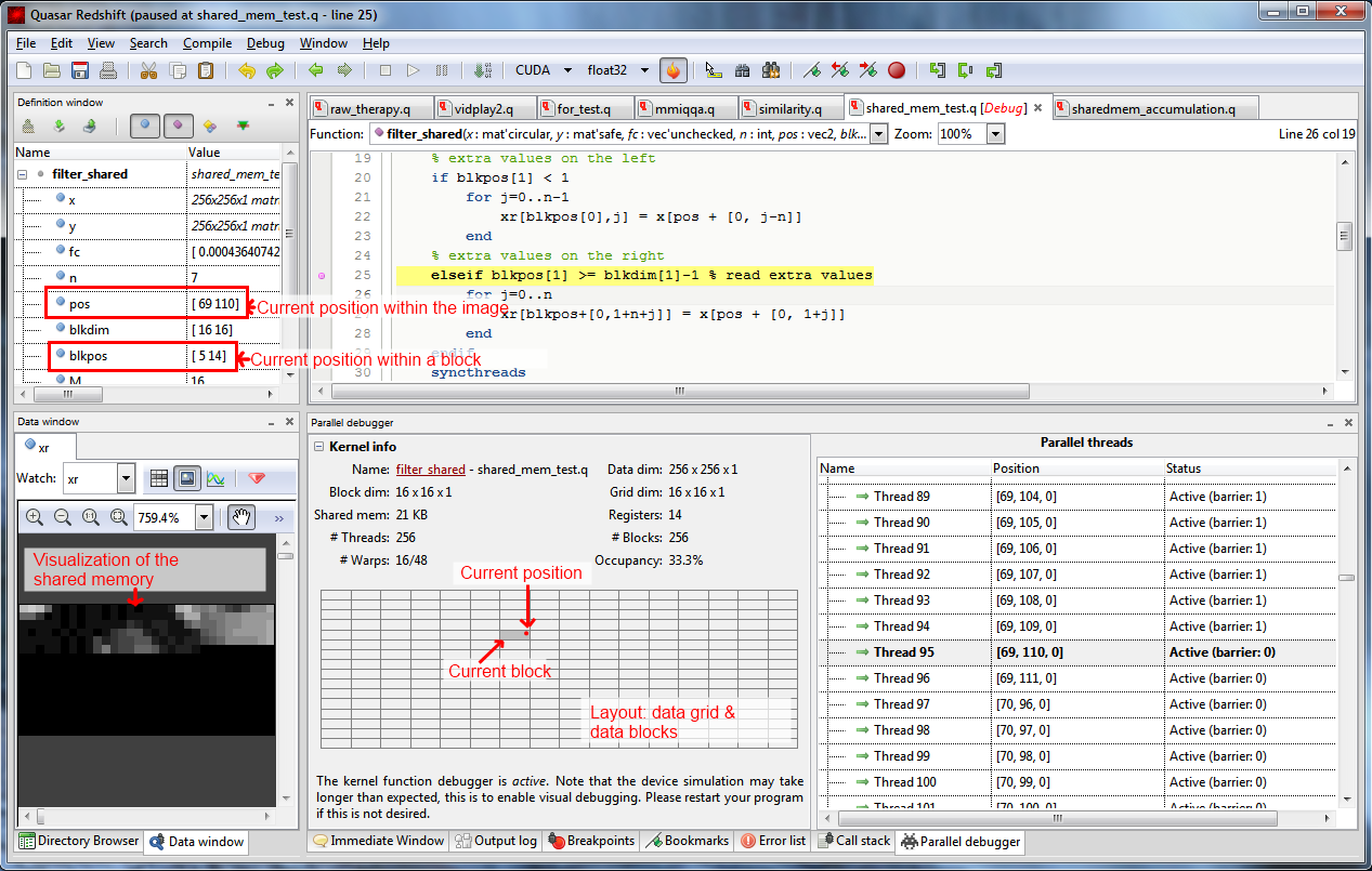
In the left pane, you see a visualization of the shared memory (through the variable xr), as well as the current position and block position variables (pos and blkpos, respectively). In the middle pane at the bottom, some information about the kernel function is given. The occupancy is an indicator of the performance of the kernel function (for example, a low occupancy may be caused by selecting block sizes that are too small). Occupancy alone however, does not give a full picture: there exist kernel function designed to achieve a low occupancy, but offering very high throughput (see for example the Volkov GTC 2010 talk).
In the right pane, an overview of the scheduled blocks and active threads is given. For active threads, the barrier index is also given: barrier 0 corresponds to all statements before the first barrier, barrier 1 corresponds to statements between the first and second barrier, and so on. Using the context menu of the list box, it is possible to switch to an other thread or to put a breakpoint at a given block.
The parallel debugger allows you to:
- Step through the kernel function (e.g. using F8 or shift-F8) [code editor]
- Place (conditional) breakpoints in kernel functions [code editor]
- Traverse different positions in the data array (or pixels in an image) [parallel debugger pane]
- Jump to the next thread/block [parallel debugger pane]
- See which threads are currently active/inactive [parallel debugger pane]
- Inspect the values of all variables that are used inside a kernel function [variable watch]
- Visualize the content of the shared memory [variable watch]
- Record videos of the kernel function in action [variable watch]
The statement evaluation order is not necessarily linear, especially in case thread synchronization is used (through syncthreads). syncthreads places a barrier, which all threads within a block must have encountered, before continuing to the next block.
Internally, kernel functions are interpreted on the CPU, in order to allow full inspection of all variables, placing breakpoints at arbitrary position within a block etc. Moreover, for clarity, the threads in between two barriers are executed serially. When a barrier (or the end of the kernel function) is met, the debugger switches to the next available thread.
The serial execution definitely makes it easy to follow what your program is doing, however in case of data races, it may also hide potential memory access conflicts (due to serialization). For this reason, there is also an option to “mimic parallel execution”, in which random thread context switches are made.
# January 2014 - new features
This documents lists a number of new features that were introduced in Quasar in Jan. 2014.
Object-oriented programming
The implementation of object-oriented programming in Quasar is far from complete, however there are a number of new concepts:
Unification of static and dynamic classes:
Before, there existed static class types (
type myclass : {mutable} class) and dynamic object types (myobj = object()). In many cases the set of properties (and corresponding types) forobject()is known in advance. To enjoy the advantages of the type inference, there are now also dynamic class types:type Bird : dynamic class name : string color : vec3 endtypeThe dynamic class types are similar to classes in Python. At run-time, it is possible to add fields or methods:
 bird = Bird()
 bird.position = [0, 0, 10]
 bird.speed = [1, 1, 0]
 bird.is_flying = false
 bird.start_flying = () -> bird.is_flying = true
Alternatively, member functions can be implemented statically (similar to mutable or immutable classes):
 function [] = start_flying(self : bird)
     self.is_flying = true
 endfunction
Dynamic classes are also useful for interoperability with other languages, particularly when the program is run within the Quasar interpreter. The dynamic classes implement MONO/.Net dynamic typing, which means that imported libraries (e.g. through
import "lib.dll") can now use and inspect the object properties more easily.Dynamic classes are also frequently used by the UI library (
Quasar.UI.dll). Thanks to the static typing for the predefined members, efficient code can be generated.One limitation is that dynamic classes cannot be used from within
__kernel__or__device__functions. As a compensation, the dynamic classes are also a bit lighter (in terms of run-time overhead), because there is no multi-device (CPU/GPU/…) management overhead. It is known a priori that the dynamic objects will “live” in the CPU memory.Also see Github issue #88 for some earlier thoughts.
Parametric types
In earlier versions of Quasar, generic types could be obtained by not specifying the types of the members of a class:
 type stack : mutable class
     tab
     pointer
 endtype
However, this limits the type inference, because the compiler cannot make any assumptions w.r.t. the type of
taborpointer. When objects of the typestackare used within a for-loop, the automatic loop parallelizer will complain that insufficient information is available on the types oftabandpointer.To solve this issue, types can now be parametric:
 type stack[T] : mutable class
     tab : vec[T]
     pointer : int
 endtype
An object of the type
stackcan then be constructed as follows:obj = stack[int]() obj = stack[stack[cscalar]]()Parametric classes are similar to template classes in C++. For the Quasar back-ends, the implementation of parametric types is completely analogous as in C++: for each instantiation of the parametric type, a
structis generated.It is also possible to define methods for parametric classes:
 function [] = __device__ push[T](self : stack[T], item : T)
     cnt = (self.pointer += 1) % atomic add for thread safety
     self.tab[cnt - 1] = item
 endfunction
Methods for parametric classes can be
__device__functions as well, so that they can be used on both the CPU and the GPU. In the future, this will allow us to create thread-safe and lock-free implementations of common data types, such as sets, lists, stacks, dictionaries etc. within Quasar.The internal implementation of parametric types and methods in Quasar (i.e. the runtime) uses a combination of erasure and reification.
Inheritance
Inherited classes can be defined as follows:
 type bird : class
     name : string
     color : vec3
 endtype

 type duck : bird
     ...
 endtype
Inheritance is allowed on all three class types (mutable, immutable and dynamic).
Note: multiple inheritance is currently not supported. Multiple inheritance has the problem that special “precedent rules” are required to determine with method is used when multiple instances define a certain method. In a dynamical context, this would create substantial overhead.
Constructors
Defining a constructor is based on the same pattern that we used to define methods. For the above stack class, we have:
 % Default constructor
 function y = stack[T]()
     y = stack[T](tab:=vec[T](100), pointer:=0)
 endfunction

 % Constructor with int parameter
 function y = stack[T](capacity : int)
     y = stack[T](tab:=vec[T](capacity), pointer:=0)
 endfunction

 % Constructor with vec[T] parameter
 function y = stack[T](items : vec[T])
     y = stack[T](tab:=copy(items), pointer:=0)
 endfunction
Note that the constructor itself creates an instance of the type, rather than that it is done automatically. Consequently, it is possible to return a
nullvalue as well.function y : ^stack[T] = stack[T](capacity : int) if capacity > 1024 y = nullptr % Capacity too large, no can do... else y = stack[T](tab:=vec[T](capacity), pointer:=0) endif endfunctionIn C++ / Java this is not possible: the constructor always returns the
this-object. This is often seen as a disadvantage.A constructor that is intended to be used on the GPU (or CPU in native mode), can then simply be defined by adding the
__device__modifier:function y = __device__ stack[T](items : vec[T]) y = stack[T](tab:=copy(items), pointer:=0) endfunctionNote #1: instead of
stack[T](), we could have used any other name, such asmake_stack[T](). Using the type name to identify the constructor:- the compiler will know that this method is intended to be used to create objects of this class
- non-uniformity (
new_stack[T](),make_stack[T](),create_stack()…) is avoided.
Note #2: there are no destructors (yet). Because of the automatic memory management, this is not a big issue right now.
Type inference enhancements
Looking ‘through’ functions (type reconstruction)
In earlier releases, the compiler could not handle the determination of the return types of functions very well. This could lead to some problems with the automatic loop parallelizer:
 function y = imfilter(x, kernel)
     ...
 endfunction  % Warning - type of y unknown

 y = imfilter(imread("x.png")[:,:,1])
 assert(type(y,"scalar"))  % Gives compilation error!
Here, the compiler cannot determine the type of
y, even though it is known thatimread("x.png")[:,:,1]is a matrix.In the newest version, the compiler attempts to perform type inference for the
imfilterfunction, knowing the type ofy. This does not allow to determine the return type ofimfilterin general, but it does for this specific case.Note that type reconstruction can create some additional burden for the compiler (especially when the function contains a lot of calls that require recursive type reconstruction). However, type reconstruction is only used when the type of at least one of the output parameters of a function could not be determined.
Members of dynamic objects
The members of many dynamic objects (e.g.
qform,qplot) are now statically typed. This also greatly improves the type inference in a number of places.
High-level operations inside kernel functions
Automatic memory management on the computation device is a new feature that greatly improves the expressiveness of Quasar programs. Typically, the programmer intends to use (non-fixed length) vector or matrix expressions within a for-loop (or a kernel function). Up till now, this resulted in a compilation error “function cannot be used within the context of a kernel function” or “loop parallelization not possible because of function XX”. The transparent handling of vector or matrix expressions with in kernel functions requires some special (and sophisticated) handling at the Quasar compiler and runtime sides. In particular: what is needed is dynamic kernel memory. This is memory that is allocated on the GPU (or CPU) during the operation of the kernel. The dynamic memory is disposed (freed) either when the kernel function terminates or at a later point.
There are a few use cases for dynamic kernel memory:
When the algorithm requires to process several small-sized (
3x3) to medium-sized (e.g.64x64) matrices. For example, a kernel function that performs matrix operations for every pixel in the image. The size of the matrices may or may not be known in advance.Efficient handling of multivariate functions that are applied to (non-overlapping or overlapping) image blocks.
When the algorithm works with dynamic data structures such as linked lists, trees, it is also often necessary to allocate “nodes” on the fly.
To use some sort of “/scratch” memory that does not fit into the GPU shared memory (note: the GPU shared memory is 32K, but this needs to be shared between all threads - for 1024 threads this is 32 bytes private memory per thread). Dynamic memory does not have such a stringent limitation. Moreover, dynamic memory is not shared and disposed either 1) immediately when the memory is not needed anymore or 2) when a GPU/CPU thread exists. Correspondingly, when 1024 threads would use 32K each, this will require less than 32MB, because the threads are logically in parallel, but not physically.
In all these cases, dynamic memory can be used, simply by calling the zeros, ones, eye or uninit functions. One may also use slicing operators (A[0..9, 2]) in order to extract a sub-matrix. The slicing operations then take the current boundary access mode (e.g. mirroring, circular) into account.
Examples
The following program transposes 16x16 blocks of an image, creating a cool tiling effect. Firstly, a kernel function version is given and secondly a loop version. Both versions are equivalent: in fact, the second version is internally converted to the first version.
Kernel version
function [] = __kernel__ kernel (x : mat, y : mat, B : int, pos : ivec2)
    r1 = pos[0]*B..pos[0]*B+B-1   % creates a dynamically allocated vector
    r2 = pos[1]*B..pos[1]*B+B-1   % creates a dynamically allocated vector

    y[r1, r2] = transpose(x[r1, r2]) % matrix transpose
                                     % creates a dynamically allocated vector
endfunction

x = imread("lena_big.tif")[:,:,1]
y = zeros(size(x))
B = 16 % block size
parallel_do(size(x,0..1) / B,x,y,B,kernel)
Loop version
x = imread("lena_big.tif")[:,:,1]
y = zeros(size(x))
B = 16 % block size

#pragma force_parallel
for m = 0..B..size(x,0)-1
    for n = 0..B..size(x,1)-1
        A = x[m..m+B-1,n..n+B-1]   % creates a dynamically allocated vector
        y[m..m+B-1,n..n+B-1] = transpose(A)   % matrix transpose
    endfor
endfor
Memory models
To acommodate the widest range of algorithms, two memory models are currently provided (some more may be added in the future).
Concurrent memory model In the concurrent memory model, the computation device (e.g. GPU) autonomously manages a separate memory heap that is reserved for dynamic objects. The size of the heap can be configured in Quasar and is typically 32MB.
The concurrent memory model is extremely efficient when all threads (e.g. > 512) request dynamic memory at the same time. The memory allocation is done by a specialized parallel allocation algorithm that significantly differs from traditional sequential allocators.
For efficiency, there are some internal limitations on the size of the allocated blocks:
The minimum size is 1024 bytes (everything smaller is rounded up to 1024 bytes)
The maximum size is 32768 bytes
For larger allocations, please see the cooperative memory model. The minimum size also limits the number of objects that can be allocated.
Cooperative memory model
In the cooperative memory model, the kernel function requests memory directly to the Quasar allocator. This way, there are no limitations on the size of the allocated memory. Also, the allocated memory is automatically garbage collected.
Because the GPU cannot launch callbacks to the CPU, this memory model requires the kernel function to be executed on the CPU.
Advantages:
- The maximum block size and the total amount of allocated memory only depend on the available system resources.
Limitations:
- The Quasar memory allocator uses locking (to limited extend), so simultaneous memory allocations on all processor cores may be expensive.
- The memory is disposed only when the kernel function exists. This is to internally avoid the number of callbacks from kernel function code to host code. Suppose that you have a
1024x1024grayscale image that allocates 256 bytes per thread. Then this would require1GBof RAM! In this case, you should use the cooperative memory model (which does not have this problem).
Selection between the memory models.
Features
Device functions can also use dynamic memory. The functions may even return objects that are dynamically allocated.
The following built-in functions are supported and can now be used from within kernel and device functions:
  zeros, czeros, ones, uninit,
  eye, copy, reshape, repmat, shuffledims, seq, linspace,
  real, imag, complex,
  mathematical functions
  matrix/matrix multiplication
  matrix/vector multiplication
Performance considerations
Global memory access: code relying on dynamic memory may be slow (for linear filters on GPU: 4x-8x slower), not because of the allocation algorithms, but because of the global memory accesses. However, it all depends on what you want to do: for example, for non-overlapping block-based processing (e.g., blocks of a fixed size), the dynamic kernel memory is an excellent choice.
Static vs. dynamic allocation: when the size of the matrices is known in advanced, static allocation (e.g. outside the kernel function may be used as well). The dynamic allocation approach relieves the programmer from writing code to pre-allocate memory and calculating the size as a function of the size of the data dimensions. The cost of calling the functions
uninit,zerosis negligible to the global memory access times (one memory allocation is comparable to 4-8 memory accesses on average - 16-32 bytes is still small compared to the typical sizes of allocated memory blocks). Because dynamic memory is disposed whenever possible when a particular threads exists, the maximum amount of dynamic memory that is in use at any time is much smaller than the amount of memory required for pre-allocation.Use
vecXtypes for vectors of length 2 to 16 whenever your algorithm allows it. This completely avoids using global memory, by using the registers instead. Once a vector of length 17 is created, the vector is allocated as dynamic kernel memory.Avoid writing code that leads to thread divergence: in CUDA, instructions execute in warps of 32 threads. A group of 32 threads must execute (every instruction) together. Control flow instructions (
if,match,repeat,while) can negatively affect the performance by causing threads of the same warp to diverge; that is, to follow different execution paths. Then,the different execution paths must be serialized, because all of the threads of a warp share a program counter. Consequently, the total number of instructions executed for this warp is increased. When all the different execution paths have completed, the threads converge back to the same execution path.
To obtain best performance in cases where the control flow depends on the block position (blkpos), the controlling condition should be written so as to minimize the number of divergent warps.
Nested parallelism
It is desired to specify parallelism in all stages of the computation. For example, within a parallel loop, it must be possible to declare another parallel loop etc. Up till now, parallel loops could only be placed at the top-level (in a host function), and multiple levels of parallelism had to be expressed using multi-dimensional perfect for loops. A new feature is that __kernel__ and __device__ functions can now also use the parallel_do (and serial_do) functions. The top-level host function may for example spawn 8 threads, from which every of these 8 threads spans again 64 threads (after some algorithm-specific initialization steps). There are several advantages of this approach:
- More flexibility in expressing the algorithms
- The nested kernel functions are (or will be) mapped onto CUDA dynamic parallelism on Kepler devices such as the GTX 780, GTX Titan. (Note: requires one of these cards to be effective).
- When a
parallel_dois placed in a__device__function that is called directly from the host code (CPU computation device), theparallel_dowill be accelerated using OpenMP. - The high-level matrix operations from the previous section are automatically taking advantage of the nested parallelism.
Notes: * There is no guarantee that the CPU/GPU will effectively perform the nested operations in parallel. However, future GPUs may be expected to become more efficient in handling parallelism on different levels.
Limitations: * Nested kernel functions may not use shared memory (they can access the shared memory through the calling function however), and they may also not use thread sychronization. * Currently only one built-in parameter for the nested kernel functions is supported: pos (and not blkpos, blkidx or blkdim).
Example
The following program showcases the nested parallelism, the improved type inference and the automatic usage of dynamic kernel memory:
function y = gamma_correction(x, gamma)
    y = uninit(size(x))

    % Note: #pragma force_parallel is required here, otherwise
    % the compiler will just use dynamic typing.
    #pragma force_parallel
    for m=0..size(x,0)-1
        for n=0..size(x,1)-1
            for k=0..size(x,2)-1
                y[m,n,k] = 512 * (x[m,n,k]/512)^gamma
            endfor
        endfor
    endfor
endfunction

function [] = main()
    x = imread("lena_big.tif")
    y = gamma_correction(x, 0.5)

    #pragma force_parallel
    for m=0..size(y,0)-1
        for c=0..size(y,2)-1
            row = y[m,:,c]
            y[m,:,c] = row[numel(row)-1..-1..0]
        endfor
    endfor

    imshow(y)
endfunction
The pragma’s are just added here to illustrate that the corresponding loops need to be parallelized, however, using this pragma is optionally. Note: * The lack of explicit typing in the complete program (even type T is only an unspecified type parameter) * The return type of gamma correction is also not specified, however the compiler is able to deduce that type(y,"cube") is true. * The second for-loop (inside the main function), uses slicing operations (: and ..). The assignment row=y[m,:,c] leads to dynamic kernel memory allocation. * The vector operations inside the second for-loop automatically express nested parallelism and can be mapped onto CUDA dynamic parallelism. # Multicomponent GPU Hardware Textures and surface writes: Improve Performance up to 2x!
Quasar supports Multicomponent GPU hardware textures. Currently, GPU textures are supported by using the following modifiers:
hwtex_nearest: nearest neighbor interpolationhwtex_linear: linear interpolation
By default, GPU textures use 32-bit floating point format (note: double precision mode is not supported by the hardware). It works as follows:
===========================================
| GPU                                     |
| ________________       ________________ |
| |Linear memory |  ===> |Texture memory| |
| ----------------       ================ |
|                                         |
===========================================
Quasar uses the linear memory as much as possible, because this offers the most flexibility: the hardware considers the data as a regular stream of bytes, without knowledge of the format.
Texture memory has predefined dimensions (width, height, depth), data type and number of components. Texture memory is stored in a non-continuous way, typically using a space-filling curve to improve cache behaviour for 2D or 3D access patterns (e.g. local windows).
Advantages of texture memory:
- Texture memory is cached, this is helpful when global memory is the main bottleneck.
- Texture memory is efficient also for less regular access patterns
- Supports linear/bilinear and trilinear interpolation in hardware
- Supports boundary accessing modes (
mirror,circular,clampedandsafe) in hardware.
By using the hwtex_nearest and hwtex_linear attributes, the compiler will generate code that uses the GPU texture lookup functions explicitly (tex1D, tex2D, tex3D) and the run-time will take care of the automatic transfers from linear memory to texture memory.
However, much more can be done to take advantage of the texture memory:
16-bit half precision floating point textures
To reduce the bandwidth in computation heavy applications (e.g. real-time video processing), it is now possible to specify that the GPU texturing unit should use 16-bit floating point formats. This can be configured on a global level in Redshift / Program Settings / Runtime / Use CUDA 16-bit floating point textures. Obviously, this will reduce the memory bandwidth by a factor of 2 in 32-bit float precision mode, and by a factor of 4 in 64-bit float precision mode.
Multi-component textures
Very often, the kernel function access RGB color data using slicing operations, such as:
x[pos[0],pos[1],0..2]When x is declared with hwtex_nearest and hwtex_linear, the compiler will complain that x[pos[0],pos[1],0..2] needs to be broken up into:
[x[pos[0],pos[1],0], x[pos[0],pos[1],1], x[pos[0],pos[1],2]]It is not a case of laziness of the compiler, but to indicate to the user that the memory access pattern is costly: instead of fetching 3 values at the same time, the three texture fetches are needed (~3 times as slow as without hardware texturing).
This can be avoided using multi-component textures:
function y = gaussian_filter_hor(x, fc, n)

    function [] = __kernel__ kernel(x : cube'hwtex_nearest(4), y : cube'unchecked, fc : vec'unchecked, n : int, pos : vec2)
        sum = [0.,0.,0.]
        for i=0..numel(fc)-1
            sum = sum + x[pos[0],pos[1]+i-n,0..2] * fc[i]
        end
        y[pos[0],pos[1],0..2] = sum
    endfunction

    y = uninit(size(x))
    parallel_do (size(y,0..1), x, y, fc, n, kernel)
endfunction
Note the parameter of hwtex_nearest(4), that specifies that 4 components need to be used. The hardware only supports 1, 2 or 4 components. In this mode, the Quasar compiler will support the texture fetching operation x[pos[0],pos[1]+i-n,0..2] and will translate the slice indexer into a 4-component texture fetch.
Result: for 16-bit floating point formats, this requires a transfer of 64 bits (8 bytes) from the texture memory (which has on most devices, its own cache that is separate from the global memory).
On average, this will reduce the memory bandwidth by a factor 2. Because of the boundary handling done by the hardware the performance may be expected to improve by even more than a factor of 2!
Remarks:
You can use 2 or 4 components in combination with images of size:
  zeros(M,N,2)
  zeros(M,N,3)
  zeros(M,N,4)
The Quasar run-time will pad the components with zeros in case the image has less color components than what you specify.
The two-component pattern may also be useful in certain cases (pairs of coefficients that are always addressed using the same indices).
Two and four component textures also fully support hardware linear interpolation and boundary handling!
For floating point textures, the texture width is no longer required to be multiple of 32 currently! Any texture dimension is accepted, as long as it is smaller than the maximum texture size supported by the hardware (e.g., for a Geforce GTX780M GPU this is
65536x65536for 2D textures and4096x4096x4096for 3D textures). The maximum texture dimensions can be retrieved by executingquasar --version.For non-floating point textures (e.g.,
mat[uint8]'hwtex_nearest), the texture width is currently still required to be a multiple of 32. This is because of hardware memory alignment requirements. In future versions of Quasar, this may change.
Example timing:
2D separable Gaussian filtering, 100x on 512x512 RGB image, 16-bit floating point texture format
Direct separable implementation: 193.011 ms
Direct separable implementation - automatic shared memory: 134.0076 ms
Direct separable implementation with multi-component GPU hardware textures: 88.005 ms
Surface writes
Since recently, it is also possible to write to texture memory, for CUDA devices with compute capability 2.0 or higher.
It suffices to declare the kernel function parameter using the modifier 'hwtex_nearest (or hwtex_nearest(n)) and to write to the corresponding matrix.
One caveat is that the texture write is only visible starting from the next kernel function call. Consider the following example:
function [] = __kernel__ kernel (y: mat'hwtex_nearest, pos : ivec2)
    y[pos] = y[pos] + 1
    y[pos] = y[pos] + 1 % unseen change
endfunction
y = zeros(64,64)
parallel_do(size(y),y,kernel)
parallel_do(size(y),y,kernel)
print mean(y) % Result is 2 (instead of 4) because the surface writes
              % are not visible until the next call
This may be counterintuitive, but this allows the texture cache to work properly.
An example with 4 component surface writes is given below (one stage of a wavelet transform in the vertical direction):
function [] = __kernel__ dwt_dim0_hwtex4(x : cube'hwtex_nearest(4), y : cube'hwtex_nearest(4), wc : mat'hwconst, ctd : int, n : int, pos : ivec2)
    K = 16*n + ctd
    a = [0.0,0.0,0.0,0.0]
    b = [0.0,0.0,0.0,0.0]
    tilepos = int((2*pos[0])/n)
    j0 = tilepos*n
    for k=0..15
        j = j0+mod(2*pos[0]+k+K,n)
        u = x[j,pos[1],0..3]
        a = a + wc[0,k] * u
        b = b + wc[1,k] * u
    endfor
    y[j0+mod(pos[0],int(n/2)),    pos[1],0..3]=a
    y[j0+int(n/2)+mod(pos[0],int(n/2)),pos[1],0..3]=b
endfunction

im = imread("lena_big.tif")
im_out = uninit(size(im))
parallel_do([size(im_out,0)/2,size(im_out,1)],im2,im_out,sym8,4,size(im_out,0), dwt_dim0_hwtex4)
On a Geforce GTX 780M, the computation times for 1000 runs are as follows:
without 'hwtex_nearest(4): 513 ms
with    'hwtex_nearest(4): 176 ms
So we obtained a speedup of approx. a factor 3 (!)
CUDA - Exploiting Constant Memory
The fact that data is constant can be exploited to yield improved kernel function performance. The GPU hardware provides several caches or memory types that are designed for this purpose:
Constant memory: NVIDIA GPUs provide 64KB of constant memory that is treaded differently from standard global memory. In some situations, using constant memory instead of global memory may reduce the memory bandwidth (which is beneficial for kernels). Constant memory is also most effective when all threads access the same value at the same time (i.e. the array index is not a function of the position).
Texture memory: texture memory is yet another type of read-only memory. With the advent of CUDA, the GPU’s sophisticated texture memory can also be used for general-purpose computing. Although originally designed for OpenGL and DirectX rendering, texture memory has properties that make it very useful for computing purposes. Like constant memory, texture memory is cached on chip, so it may provide higher effective bandwidth than obtained when accessing the off-chip DRAM. In particular, texture caches are designed for memory access patterns exhibiting a great deal of spatial locality.
For practical purposes, the size of the constant memory is rather small, so it is mostly useful for storing filter coefficients and weights that do not change while the kernel is executed. On the other hand, the texture memory is quite large, has its own cache, and can be used for storing constant input signals/images.
The drawback is that the texture memory is separate from the global memory and can not be written. As such, global memory needs to be copied to texture memory before the kernel is started. This way, sometimes two separate copies of the data need to be stored in the GPU memory. Luckily, for Kepler GPUs, there is a solution (see further 'hwtex_const).
In Quasar, constant/texture memory can be utilized by adding modifiers to the kernel function parameter types. The following modifiers are available:
'hwconst: the vector/matrix needs to be stored in the constant memory. Note: if there is not enough constant memory available, a run-time error is generated!'hwtex_nearestor'hwtex_linear: the vector/matrix needs to be stored in the texture memory'hwtex_const- non-coherent texture cache. This option requires CUDA compute architecture 3.5 or higher - as in Geforce GPUs of the 900 series, and allows the data still be stored in the global memory, will utilizing the texture cache for load operations. This combines the advantages of the texture memory cache with the flexibility (ability to read/write) of the global memory. Note: internally,hwtex_constis implemented using the__ldg()intrinsic.
Note that global memory accesses (i.e., without 'hw* modifiers) are cached in L2. For Kepler GPU devices, using 'hwtex_const the texture cache is utilized directly, bypassing the L2 cache. The texture cache is a separate cache with a separate memory pipeline and relaxed memory coalescing rules, which may bring advantages to bandwidth-limited kernels. Source: Kepler tuning guide.
Starting with Maxwell GPU devices, the L1 cache and the texture caches are unified. The unified L1/texture cache coalesces the memory accesses, gathering up the data requested by the threads in a warp, before delivering the data to the warp. Source: Maxwell tuning guide.
Correspondingly, some optimization tips are:
When your kernel function is using some constant vectors (weight vectors with relatively small length), and when all threads access the same value of the vector at the same time (the index is not a function of the position!), you should definitely consider using
'hwconst.When your kernel function is accessing constant images (
vec,matorcube) on Kepler/Maxwell devices with compute architecture >= 3.5 (checkquasar --version), it may be worthful to usehwtex_const.Because of the L2 cache, memory coalescing and various bandwidth factors, please don’t use
'hwconst,'hwtex_constblindly. The best is to investigate whether the modifier improves the performance (e.g. using the Quasar profiler, it is even possible to make comparison profiles). Only keep the modifiers when they improve the performance.
In the future, the Quasar compiler may be able to add 'hwconst, 'hwtex_const automatically. For now, lets start testing and understanding when these modifiers are beneficial!
Example
As an example, consider the following convolution program:
Default version with no constant memory being used:
function [] = __kernel__ kernel(x : vec, y : vec, f : vec, pos : int)
    sum = 0.0
    for i=0..numel(f)-1
        sum += x[pos+i] * f[i]
    endfor
    y[pos] = sum
endfunction
Version with constant memory:
function [] = __kernel__ kernel_hwconst(x : vec, y : vec, f : vec'hwconst, pos : int)
    sum = 0.0
    for i=0..numel(f)-1
        sum += x[pos+i] * f[i]
    endfor
    y[pos] = sum
endfunction
Version with constant texture memory for f:
function [] = __kernel__ kernel_hwtex_const(x : vec, y : vec, f : vec'hwtex_const, pos : int)
    sum = 0.0
    for i=0..numel(f)-1
        sum += x[pos+i] * f[i]
    endfor
    y[pos] = sum
endfunction
Version with constant texture memory for x and f:
function [] = __kernel__ kernel_hwtex_const2(x : vec'hwtex_const, y : vec, f : vec'hwtex_const, pos : int)
    sum = 0.0
    for i=0..numel(f)-1
        sum += x[pos+i] * f[i]
    endfor
    y[pos] = sum
endfunction
Version with HW textures:
function [] = __kernel__ kernel_tex(x : vec, y : vec, f : vec'hwtex_nearest, pos : int)
    sum = 0.0
    for i=0..numel(f)-1
        sum += x[pos+i] * f[i]
    endfor
    y[pos] = sum
endfunction
Timing code:
x = zeros(2048^2)
y = zeros(size(x))
f = 0..31  % dummy filter coefficients

tic()
for k=0..99
    parallel_do(size(y),x,y,f,kernel)
endfor
toc("Default")

tic()
for k=0..99
    parallel_do(size(y),x,y,f,kernel_hwconst)
endfor
toc("'hwconst")

tic()
for k=0..99
    parallel_do(size(y),x,y,f,kernel_hwtex_const)
endfor
toc("'hwtex_const")

tic()
for k=0..99
    parallel_do(size(y),x,y,f,kernel_hwtex_const2)
endfor
toc("'hwtex_const2")

tic()
for k=0..99
    parallel_do(size(y),x,y,f,kernel_tex)
endfor
toc("'hwtex_nearest")
Results for the NVidia Geforce 980 (Maxwell architecture):
Default: 513.0294 ms
'hwconst: 132.0075 ms
'hwtex_const: 128.0074 ms
'hwtex_const: 95.005 ms
'hwtex_nearest: 169.0096 ms
It can be seen that using constant memory alone yields a speed-up of more than factor 5(!). The best performance is obtained with hwtex_const, which is close to the performance of 'hwconst.
Note, further improvement can be made using shared memory, for which we reach 85 ms in this case.
CUDA Unified Memory
CUDA unified memory is a feature introduced in CUDA 6.0. For unified memory, one single pointer is shared between CPU and GPU. The device driver and the hardware make sure that the data is migrated automatically between host and device. This facilitates the writing of CUDA code, since no longer pointers for both CPU and GPU need to be allocated and also because the memory is transferred automatically.
In general, CUDA programs making use of unified memory are slightly (10-20%) slower than programs that perform the memory management themselves (like Quasar). However, for some programs (e.g. programs which heavily rely on recursive data structures, such as linked lists, trees and graphs) it is useful to take advantage of the unified memory, because the Quasar run-time is then relieved of the object memory management.
For now, because it is still an experimental feature, this can be achieved by setting the following option in Quasar.Runtime.Config.xml:
<setting name="RUNTIME_CUDA_UNIFIEDMEMORYMODE">
    <value>Always</value>
</setting>
To use unified memory in Quasar, there are the following requirements:
- The minimal CUDA driver version needs to be 6.0.
- Because of address space sizes, only 64-bit versions of Quasar support the unified memory, otherwise the setting has no effect.
- The Hyperion engine (v2 runtime) needs to be used.
Unified memory and multi-GPU processing
An additional advantage of unified memory is that allocations are visible to all GPUs in the system via peer-to-peer copy capabilities of the GPUs. However, when peer-to-peer connections are not available (e.g. GPUs of different architectures, GPUs connected to different IDE buses), CUDA falls back to using zero-copy memory in order to guarantee data visibility. Unfortunately, we have noted that the fallback may have a dramatic impact on the performance (to even 100x-1000x slower). Moreover, the fallback happens automatically, regardless of whether both GPUs are actually used by a program.
If only one GPU is actually going to be used, one solution is to set the CUDA_VISIBLE_DEVICES=0 environment variable before launching Quasar / Redshift. This environment sets which GPU are visible to CUDA / Quasar. On a system with two GPUs or more, with no peer-to-peer support, unified memory allocations will not fall back to zero-copy memory.
Read more in the CUDA C programming guide. # ’const and ’nocopy modifiers
The types of kernel function parameters can have the special modifiers 'const and 'nocopy. These modifiers are added automatically by the compiler after analyzing the kernel function. The meaning of this modifiers is as follows:
| Type modifier | Meaning |
|---|---|
| ’const | The vector/matrix variable is constant and only being written to |
| ’nocopy | The vector/matrix variable does not need to be copied to the device before the kernel function is called |
The advantage of these type modifiers is that it permits the run-time to avoid unnecessary memory copies between host and the device. In case of parameters with the 'const modifier, the dirty bit of the vector/matrix does not need to be set. For 'nocopy, it suffices to allocate data in device memory without initializing it.
Furthermore, the modifiers are exploited in later optimization and code generation passes, e.g. to take automatic advantage of caching capabilities of the GPU.
An example of the modifiers is given below:
function [] __kernel__ copy_kernel(x:vec'const,y:vec'nocopy,pos:int)
    y[pos] = x[pos]
endfunction
x = ones(2^16)
y = zeros(size(x))
parallel_do(numel(x),x,y,kernel)
Here 'nocopy is added because the entire content of the matrix y is overwritten.
Comparison to other modifiers
In Quasar, two other modifiers can be used for constant objects: 'hwconst and 'hwtex_const. The relation between these modifiers is as follows:
'hwconst: declares the kernel function parameter to reside in constant memory of the GPU. 'hwconst therefore implies 'const.
'hwtex_const: uses the non-coherent texture cache of the GPU for accessing the global memory. Also, 'hwconst implies 'const.
In case 'const, 'hwconst, or 'hwtex_const are used for non-constant variables, the compiler will generate an error.
Multi GPU Support
From now on, the Hyperion engine offers support for multiple GPUs and the run-time “intelligence” is improving with every new Quasar release!
Concurrency over multiple GPUs imposed a few challenges to the Quasar run-time. First: having one controlling thread per GPU, or controlling all GPUs from one single thread. The former is preferable when the GPUs are doing truly independent work but becomes a bit more tricky when the GPUs need to co-operate. In the latter, co-operation is facilitated but then we must ensure that all GPUs get enough workload so that not the controlling thread with inherent synchronization becomes the bottleneck.
To enable the “synchronous” host programming model of Quasar (i.e., as seen by the programmer), the second technique is used by the Hyperion engine.
In fact, the multi-GPU feature entirely relies on the concurrent kernel execution possibilities (turbo mode) of Quasar. The turbo mode further uses the asynchronous CUDA API functions, but also extends the asynchronous processing to the CPU. In the background, dependencies between matrix variables, kernels etc. are being tracked and the individual memory copy operations and kernel calls are automatically dispatched to one of the available CUDA streams. This way, operations can be performed in parallel on the available GPU hardware. At appropriate places, sychronization points are created, for example, to transfer data from one GPU to another GPU. These synchronization points only mutually affect the GPUs, but not the CPU. This means that at the same time, the CPU can continue its work, like scheduling new commands for the GPUs, or performing “smaller” work for the GPUs. In the Hyperion engine, it is even possible (and common) to have three CPU threads, from which one controls the GPUs and two others are able to perform independent work (for example like small matrix calculations for each of the GPUs).
So despite the fact that the programming model is synchronous, the underlying implementation certainly isn’t!
Peer to peer memory copies and host-pinnable memory
For optimal cooperation between multiple GPUs, it is best that the GPUs have peer-to-peer capabilities. In practice, this means that the GPUs need to be connected to the same PCIe bus, so that memory transfers from one GPU to another GPU are direct (bypassing the CPU host memory). The Hyperion engine automatically checks which GPUs have peer-to-peer capabilities. When these capabilities are not present, copying is performed via the non-pageable (also called host-pinnable) system memory. This is system memory that cannot be swapped to disk (as virtual memory), but that permits direct memory access (DMA) from the GPU. Copying via host-pinnable memory is generally faster than with pageable memory, but also permits asychronous memory copies from the GPU to the host (without host-pinnable memory these memory copies are blocking!).
One disadvantage of host pinnable memory, is that takes physical RAM away from other programs: the memory is locked and cannot be swapped from disk. According to the CUDA documentation, in extreme cases in which, say >75% of the total memory is pinned, this may cause irresponsiveness of the OS. Therefore, the use of CUDA host pinnable memory currently needs to be enabled via the device config file:
<cpu-device num-threads="2" cuda-hostpinnable-memory="true" />Multi-GPU device configuration file
A typical device config file looks as follows:
<quasar>
    <computation-engine name="Dual GeForce GTX 980 engine" short-name="CUDA - dual">
        <cpu-device num-threads="2" max-cmdqueue-size="96" cuda-hostpinnable-memory="true" />
        <cuda-device max-concurrency="4" max-cmdqueue-size="1024" ordinal="0" />
        <cuda-device max-concurrency="4" max-cmdqueue-size="1024" ordinal="1" />
    </computation-engine>
</quasar>
Here, the CPU device has two threads for performing tasks. Note that each thread can again spawn several sub-threads (e.g. via OpenMP). For example, on an 8-core processor, each of the threads will be subdivided into 4 threads that are used with OpenMP. The idea is then that each of the 2 CPU threads works for one GPU individually (by performing lighter kernel calls), so that the GPUs can work more or less independently. Further, each GPU has a maximal concurrency of 4, which means that the GPU can (when possible on the hardware level) execute 4 kernel functions (or memory copies) in parallel. The intra-GPU concurrency is particularly useful because it may help to further hide the memory. latencies.
Each of the devices has its own command queue, this is a queue on which the load balancer places individual commands that needs to be processed by the respective devices. To avoid the system running out of memory too quickly (imagine a commander that is giving orders 10x faster than the soldiers can follow), there is a maximum size of the command queues. When the command queue is full, the host thread needs to wait until at least one space is available.
To maximally exploit the available (in)dependencies between the data and to maximize concurrency, it is best to set the maximum command size as big as possible. Here, the maximum queue size was here determined experimentally.
Load balancing
One interesting feature is that the load balancing is entirely automatic and will take advantage of the available GPUs, when possible. In some cases it is useful to have more control about which GPU is used for which task. This can be achieved by explicitly setting the GPU device via a scheduling instruction:
{!sched gpu_index=0}
or
{!sched gpu_index=1}
This overrides the default decision of the load balancer. For for-loops this can be done as follows:
for k=0..num_tasks-1
    {!sched gpu_index=mod(k,2)}
    perform_task_step1(k)
    perform_task_step2(k)
endfor
This way, each GPU will take care of one iteration of the loop. To help the run-time system, and to avoid the command queue from overrunning while one GPU is idle, it may be more beneficial to use the following technique
for k=0..num_tasks-1
    {!unroll times=2; multi_device=true}
    perform_task_step1(k)
    perform_task_step2(k)
endfor
This way, the compiler will unroll the loop by a factor 2 (corresponding to the number of GPUs in the system) and generate the following code:
for k=0..2..num_tasks-1
    {!sched gpu_index=0}
    perform_task_step1(k)
    {!sched gpu_index=1}
    perform_task_step1(k+1)

    {!sched gpu_index=0}
    perform_task_step2(k)
    {!sched gpu_index=1}
    perform_task_step2(k+1)
endfor
The more regular switching between both GPUs is often more efficient because it makes sure that both GPUs are busy. An example obtained using the NVidia nSight profiler is given below:
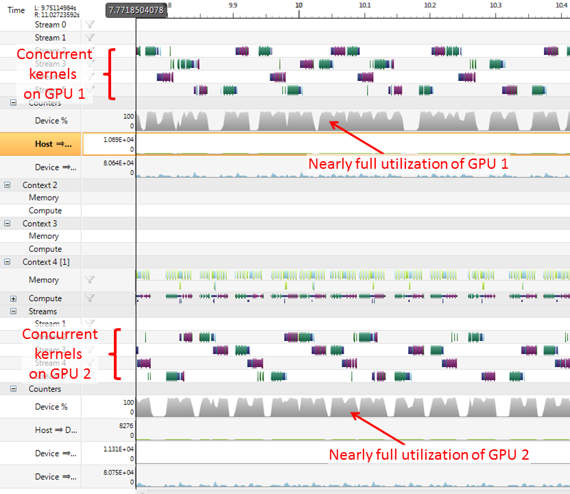
It can be seen that, despite the complex interactions on different streams, the GPUs are kept reasonably busy with these load balancing techniques.
Warning: Note that to benefit from the multi-GPU acceleration over single-GPU use, it is important to keep the GPUs sufficiently busy. If the kernel functions process small data sets, then the bottleneck may still be on the CPU side and the application will not see a lot of speedups!
A simple multi-GPU processing example
Below we give a simple multi-GPU processing example. Only one line was added to manually distribute the workload over the two GPUs.
function [] = __kernel__ filter_kernel(x:cube,y:cube,offset:ivec3,pos:ivec3)
    dpos = pos+offset;
    M = 9
    sum = 0.0
    for m=-M..M
        for n=-M..M
            sum += x[dpos+[m,n,0]]
        endfor
    endfor
    y[pos] = sum ./ (2*M+1)^2
endfunction

function [] = main()

    im = imread("lena_big.tif")

    % Loop unrolling for multi-GPU processing
    tic()
    for k=0..99
        {!sched gpu_index=mod(k,2)}
        offset = k*size(im,0)/16
        im_out = uninit(size(im))
        parallel_do([size(im,0)/16,size(im,1),size(im,2)], im, im_out, [offset,0,0], filter_kernel)
    endfor
    toc()
    {!sched gpu_index=0}

    imshow(im_out)

endfunction
Comments on an additional feature: CUDA 6.0 Unified memory
CUDA unified memory is a feature introduced in CUDA 6.0. For unified memory, one single pointer is shared between CPU and GPU. The device driver and the hardware make sure that the data is migrated automatically between host and device. The same happens when multiple GPUs are involved: the run-time system only sees one pointer that can be used on CPU or on either GPU. Of course, this requires 64-bit addressing spaces and is only available in 64-bit versions of Quasar. Unified memory reduces the run-time overhead at Quasar level and moves it to the driver level (although in our experiments, programs making use of unified memory are often slightly (10-20%) slower than without unified memory).
Unified memory can be enabled by setting in Quasar.Runtime.config.xml:
<setting name="RUNTIME_CUDA_UNIFIEDMEMORYMODE">
    <value>Always</value>
</setting>
However, there is one caveat: using unified memory in a multi-GPU configuration requires peer-to-peer capabilities of the GPUs. If peer mappings are not available (for example, between GPUs of different architectures), then the system will fall back to using zero-copy memory in order to guarantee data visibility. This fallback happens automatically, regardless of whether both GPUs are actually used by a program. This practically means that no memory is allocated on the GPU, all memory allocations in the CPU memory, and the memory is accessed via DMA, dramatically impacting the performance (often 100x-1000x slower!).
Therefore, it is best to not use unified memory when peer-to-peer capabilities are not available. Alternatively it can be useful to set the CUDA_VISIBLE_DEVICES environment variable before launching the program, so that only GPUs with peer-to-peer capabilities are selected. This constrains which GPUs are visible. Read more at: http://docs.nvidia.com/cuda/cuda-c-programming-guide/.
April 2017 - New Quasar Features
This document outlines language features added to Quasar in 2017. The new features mostly support new applications (e.g, computational mathematics, parallel data structures) or improve some existing applications.
Type system improvements
First, we list some enhancements added to the type system. The enhancements are mostly minor, but greatly improve the type inference process.
Explicitly typed lambda expressions
To help the type inference, or to ensure that the result of lambda expressions is as you define, it is now possible to specify the types of the output parameters of a lambda expression:
sinc : [scalar -> scalar] = sin(x) / xThe same approach works for higher level lambda expressions, where the type of the higher level function can directly be specified (enhancing the readability).
wrap : [mat -> vec -> mat] = A -> x -> x * transpose(A)is equivalent to
wrap = (A : mat) -> (x : vec) -> x * transpose(A)Tuple types and lambda functions with multiple output parameters
In Quasar, tuples {12,"value"} are represented by fixed-length cell matrices: in essence, a tuple is a cell matrix with a length constraint attached to it. The objects can just be constructed using the notation {...}. What is new is that the Quasar compiler can now perform type inference on these tuple types. For this purpose, the type of the above expression is represented by the following syntax:
vec[{int, string}]This indicates that the vector consists of two components: an integer and a string. Correspondingly, the type:
vec[{scalar, scalar, scalar}]is equivalent to vec3. It is also possible to define matrix tuple types:
mat[{{scalar, int}, {int, scalar}}]Of course, the purpose is here to mainly show that it is possible. For code clarity it is better to use classes for this purpose, where the fields can be explicitly named. Moreover, for most user code, it is not required to use the tuple types explicitly as they are mostly a result of the type inference. They may appear in some compiler error/warning messages.
Tuples are useful for defining lambda expressions with multiple arguments. For example,
swap : [(??,??) -> (??,??)] = _
    (x, y) -> {y, x}
By explicitly defining the type of the lambda expression, the result of the expression {y, x} can be interpreted as the return values y and x. Correspondingly, two values can be swapped by using:
[a, b] = swap(a, b)In previous versions of Quasar, it was not possible to have lambda expressions returning multiple values.
Type modifier merging
Type modifiers 'const, 'circular', 'checked' can now be used directly, without defining a variable type. The variable type will then be inferred using the standard type inference engine. For example, a constant can just be defined as:
my_constant : 'const = 2.3455Defining constants in this way has the advantage that 1) the compiler can ensure that the value of the variable is never modified and 2) the constants may directly be substituted into the kernel/device functions, which makes the use of them more efficient. This is done automatically.
Enumerations
To simplify some of the parameters (which were previously defined as strings), enums have been introduced. An enum type can be defined as follows:
type color : enum
    Red
    Green
    Blue = 4
    Cyan
    Magenta
    Yellow
endtype
where every possible value of the enum type is specified. Optionally, a value can be declared for the enum value. The compiler automatically assigns values to the enums, starting with 0, and increasing by 1 for every entry. Hence in the above example, Green = 1. When the enum value is specified in the code, the compiler continues counting at this value, so Cyan=5, Magenta=6, etc.
An enum variable can be created as follows:
a = color.RedFor matches, there is a simplified way: in case the type of a is known at compile-time, the enum type color. does not need to be specified.
match a with
| Red   -> print ("The color is red")
| Green -> print ("The color is green")
| _ -> print ("Unknown color")
endmatch
The advantage of enums over string constants is that you have direct control over the possible values of the enums. Moreover, enums can be used within kernel/device functions (which is not possible with string constants).
Exception handling
To be able to develop robust user interfaces, Quasar has now a rudimentary form of OOP-based exception handling implemented. The exception handling is not yet as refined as in e.g., java, C#, but the main functionality is operational.
Exceptions can be caught using try/catch blocks, as follows:
try
    error "I fail"
catch ex   % or catch ex : qexception
    print "Exception caught: ", ex
endtry
By default, exceptions are of the type qexception. The class qexception has a method message which allows retrieving the message of the exception. In the future, it will be possible to define custom exception classes by inheriting from qexception, also multiple catch blocks can be defined (one for every exception class).
Notes: because of GPU programming limitations, it is currently not possible to use try-catch blocks within kernel or device functions (when you attempt to, an error will be generated by the compiler). Instead, it is recommended to use implement your own error handling mechanism (for example using kernel function return values). However, it is possible to throw exceptions from a kernel function using error. These exceptions can be caught using a try-catch block in the surrounding host function.
Generic type aliases
Quasar also now supports generic type aliases, for example:
type my_cool_vector[T] : vec[vec[T]]Generic type aliases are type aliases with type parameters. They can simplify the type definitions. For example, they come in handle when defining a hashmap class.
type Hashmap_entry[K, T] : class
    key : K
    value : T
endtype

type Hashmap_bucketlist[K, T] : vec[^List[Hashmap_entry[K,T]]]

type Hashmap[K, T] : class
    buckets : Hashmap_bucketlist[K, T]
    hashkeygenerator : [K -> int]
endtype
Reduction enhancements
To allow more symbolic manipulations to be defined in Quasar programs, a few enhancements to the reduction system were necessary. These changes are described in more detail in this section.
Local reductions
Reductions can now be defined inside function scopes. Outside of the function, the reduction no longer has an effect. In combination with macros, this allows selective application of sets of reductions.
Variadic reductions
Variadic functions were introduced before, using the following syntax:
function [] = func(... args)
    for i=0..numel(args)-1
        print args[i]
    end
end
Such functions are particularly useful for passing parameters in a flexible way, e.g., as in a main function (for a main function, the command line parameters are conveniently mapped onto the variadic arguments).
In analogy to variadic functions, there are now variadic reductions, with a similar purpose. For example, a reduction can be defined for the above function:
reduction (...args : vec) -> myprint(args) = func("some text", ...args)Internally, variadic reductions are also used for implementing variadic methods:
type myclass : mutable class
    count : int
endtype

function [] = format(self : myclass, ...args : vec[??])
    print ...args, " count=", self.count
endfunction
During the reduction expansion, the variadic parameter packs are passed as a cell vector (again: we benefit from the fact that tuple types can help the type inference engine).
There are more advantages to come, read further.
Lambda capturing reductions
Lambda capturing reductions allow function variables to be captured by the reduction expression. This way, some more advanced symbolic manipulation can be performed. For example, the difference of two functions can be defined as
reduction (f : function, g : function, x) -> (f - g)(x) = x -> f(x) - g(x)
% (fn1 - fn2)(1) becomes fn1(1) - fn2(1)
With lambda capturing reductions, it is now possible to define an argmin reduction that captures parameters but also functions:
reduction (x, y, W, lambda) -> argmin(sum((y - W(x)).^2) + lambda * sum(x.^2), x) =
    my_solver(W,y,lambda)
This will be used for constructing a new mathematical optimization library for Quasar.
Variadic lambda capturing reductions
Combining the techniques from the previous two sections, we obtain variadic lambda capturing reductions:
reduction (x, ...lambda, ...f) -> sum([lambda2*(sum(f(x).^2))]) = mysum(f,lambda)
print 2*sum(x.^2) + cos(3) * sum((2*x).^2) + 2*sum((-x).^2)
Note that here, there are two sets of variadic parameters: lambda and f. The syntax sum([...]) calculates the sum of the components of a vector and correspondingly, it is recognized by the reduction system to expand summations. In particular, the above print statement reduces to:
print mysum({((x) -> x),((x) -> (2*x)),((x) -> -(x))},{2,cos(3),2})The captured functions are expanded into a cell vector of functions.
Function enhancements: unpacking of objects to optional function arguments
The function call interface also obtained an enhancement. In many applications, it is useful to pass optional parameters to functions. Optional parameters simplify function calls, as it is easy to set the default values (which can be scalars, matrices or even functions).
The spread operator ... expands a vector into its components, this reduces expressions like a[pos[0],pos[1],pos[2],0..2] to a[...pos,0..2]. Idem for cell vectors, like ...{1,2,3}. On the other hand, the syntax {a:=val1,b:=val2} creates a dynamic object (similar to the dictionary-like Python objects). Logically combining both concepts, applying the spread operator then expands the object into its individual fields ...{a:=val1,b:=val2}. This feature has now been implemented:
function [] = my_func(text, param1 = 0.2, param2 = 0.6)
    print param1, ",", param2
endfunction

arg_list = { param2 := 2, param1 := 1, other := "hello" }
my_func("param:", ...arg_list)
As expected, the function my_func will print 1,2. The argument list arg_list is filtered automatically: unsed parameters (such as other) are simply ignored. Argument lists are particularly useful when passing the same sets of arguments to multiple functions.
Loop enhancements
Multi-device for-loops
To parallelize over multiple devices (e.g., multiple GPUs), the following code attribute can be used:
{!parallel for; multi_device=true}
for index = 0..numel(items)-1
    ...
endfor
Here, the compiler will generate code to execute every iteration on a different GPU. In case the loop is not parallelizable, a dependency warning will be shown, just as with the regular loops.
Note that the multi-GPU feature requires the use of the Hyperion (v2) engine.
Imperfect for-loop parallelization (experimental feature)
Perfect parallelizable for-loops are loops that iterate over a rectangular domain, where every iteration is independent from the other. On the other hand, imperfect for-loops are not restricted to rectangular domains and can have certain dependencies between the iterations, while still permitting some form of parallelization (either completely, either partly).
The Quasar compiler can now parallelize a number of imperfect loops. To enable this feature, it is required to set the code attribute:
{!function_transform enable="imperfectloop"}The following loop:
for m=0..M-1
    for n=0..N-1
        for p=0..2
            im[m,n,p] = 0.3 * im[m-1,n-1,p] + 0.4 * im[m-2,n-2,p] + 0.3*im[m,n,p]
        end
    end
end
can then be expanded into:
function [] = __kernel__ kernel(M:int,N:int,im:cube,pos:ivec2) concealed
    n2=pos[1]-M+1
    for p2=0..M-1
        if n2+p2>=0 && n2+p2<=N-1
            im[p2,n2+p2,pos[0]]=0.3*im[p2-1,n2+p2-1,pos[0]]+
                0.4*im[p2-2,n2+p2+-2,pos[0]]+0.3*im[p2,n2+p2,pos[0]]
        endif
    endfor
endfunction

parallel_do([3.,N+M-1],M,N,im,kernel)
Hence, the outer loop is parallelized, while the inner loop is executed sequentially. Essentially a skewing of the coordinate system was performed.
Nested loop parallelism enhancements
The compiler now takes nested for-loop parallelization hints into account, effectively mapping them onto nested parallelism (OpenMP for CPU targets, dynamic parallelism for CUDA).
{!parallel for}
for m=0..size(im,0)-1
    avg = mean(im[m,:])
    {!parallel for}
    for n=0..size(im,1)-1
        im[m,n] = im[m,n] - avg
    endfor
endfor
Before, it was possible to manually define nested kernel functions. Now the compiler can also parallelize multiple levels of nested functions.
There is one limitation: for CUDA devices the inner functions can currently not have reduction/accumulation variables.
Kernel/device enhancements
Atomic exchange and atomic compare and swap
Two new operators have been added:
Atomic exchange
old_value = (variable <- new_value)The atomic exchange operator reads the old value of a variable and replaces it by a new value, in one atomic operation.
Atomic compare and swap
old_value = (variable <- (new_value, expected_value))The atomic compare and swap operator reads the old value of the variable and replaces it by a new value, but only when the old value was found to be equal to the expected value.
The atomic operators are used for defining parallel lock-free data structures, such as concurrent sets, stacks (see below!).
Note that for GPU targets, atomic compare and swap should not be used to implement mutexes, semaphores, or critical sections, because threads in a warp are executed in a lock-step, so that the use of mutexes automatically results in a deadlock!
Kernel/device functions with target-dependent optimizations
The $target() meta-function allows to detect the platform target for which a kernel/device function is compiled. Note that often, multiple versions of kernel/device functions are compiled, each for different platforms. The $target() meta-function permits influencing the code in the target-specific optimization pipelines:
function [] = __kernel__ func(pos : ivec3)
    if $target("gpu")
        % GPU specific code/optimizations come here
    else
        % CPU specific code/optimizations come here
    endif
endfunction
The following targets are available:
- cpu: a default CPU target
- gpu: a default GPU target (e.g. CUDA, OpenCL)
- nvidia_cuda: NVidia CUDA GPU target
- opencl: an OpenCL target
- nvidia_opencl: NVidia OpenCL devices
- amd_opencl: AMD OpenCL devices
The list of targets will likely increase in the future. Note that the above example, it is required that the kernel dimensions and block size are the same for each target platform. In case this is not desired, a more advanced alternative is to define the kernel functions for each platform individually (using {!kernel target="gpu"}) and to use the schedule() function to invoke the run-time scheduler manually.
Macros for specifying optimization profiles
Quasar now also has a concept of “macros”. Macros are basically functions which are evaluated at compile-time. In its most simple form, a macro is expanded completely at compile-time:
macro [] = time(op)
    tic()
    op()
    toc("Operation")
endmacro

function [] = operation()
    % Do something...
endfunction

!time operation
%or {!time operation}
The last line of code invokes the macro. That’s right: the macro invocation uses the Quasar code attribute syntax !attr. The braces around the attribute are now optional.
Another use of macros is to specify optimization profiles. These profiles give the compiler some information about how a kernel function needs to be optimized, by defining “mechanical” actions (code transformations) that need to be applied to the code. For this purpose, it is not uncommon that the macros themselves contain target-specific code ($target()). An additional advantage is that a profile can be shared between different kernel functions.
In the future, an autotuning function may be added that will allow the compiler to automatically determine the optimal parameters used by a macro.
The following example illustrates an optimized CPU/GPU implementation of a backward convolution kernel for use in convolutional neural networks. With this implementation, a speedup of ~50% was obtained compared to NVIDIA’s cuDNN library, for radius=2.
macro [] = backward_convolution_profile(radius, channels_in, channels_out, dzdw, input)
    % Generates specialized versions of the kernel function for different
    % combinations of the input parameters
    !specialize args=(radius==1 && channels_out==3 && channels_in==3 || _
                     radius==2 && channels_out==3 && channels_in==3 || _
                     radius==3 && channels_out==3 && channels_in==3 || _
                     radius==4 && channels_out==3 && channels_in==3 )

    if $target("gpu")
    % Small radii: apply some shared memory caching
    if radius <= 3
        % Calculate the amount of shared memory required by this transform
        shared_size = (2*radius+1)^2*channels_in*channels_out

        !kernel_transform enable="localwindow"
        !kernel_transform enable="sharedmemcaching"
        !kernel_arg name=dzdw, type="inout", access="shared", op="+=",
        cache_slices=dzdw[:,:,pos[2],:],numel=shared_size
        !kernel_arg name=input, type="in", access="localwindow",
        min=[-radius,-radius,0], max=[radius,radius,0], numel=2048
    endif
    !kernel_tiling dims=[128,128,1], mode="global", target="gpu"
    endif
endmacro

function [] = __kernel__ backward_convolution_kernel(dzdoutput:Data,dzdinput:Data,input:Data,dzdw:Parameter,
    w:Parameter'hwconst,radius:int,channels_in:int,channels_out:int,pos:ivec3)
    summ = zeros(channels_out)

    % Optimization profile for this kernel function!
    !backward_convolution_profile radius, channels_in, channels_out, dzdw, input

    for dy = -radius..radius
        for dx = -radius..radius
            !unroll
            for c_out  = 0..channels_out-1
                !auto_vectorize
                summ[c_out] += w[dy+radius,dx+radius,pos[2],c_out]*
        dzdoutput[pos[0]+dy,pos[1]+dx,c_out]
                dzdw[dy+radius,dx+radius,pos[2],c_out] +=
        dzdoutput[pos[0],pos[1],c_out] * input[pos[0]+dy,pos[1]+dx,pos[2]]
            endfor
        endfor
    endfor
    dzdinput[pos] = sum(summ)
endfunction
As can be seen, using macros, the optimization information can nicely be splitted from the implementation (backward_convolution_kernel). The implementation itself is fairly generic.
Branch divergence reducer
On the GPU, the threads are executed in groups of 32 called a warp. When a conditional branch occurs (e.g., for an if-else block), the GPU will sequentially evaluate the ‘if’ and the ‘else’ blocks (thereby disabling the threads for which the test condition does not hold). This is called branch divergence. Due to the sequential nature and due to the fact that threads are temporarily being disabled, this may hugely impact the performance!
Due to suggestions, I managed to collect a few code fragments for which branch divergence can easily be solved using code transformations. For this, I added the branch divergence reducer kernel transform. The transform can be enabled using:
{!kernel_transform enable="branchdivergencereducer"}An example code fragment that suffers from branch divergence:
if (input[pos] > 0)
  accumulator_pos[pos] = input[pos]
else
  accumulator_neg[pos] = input[pos]
endif
After transformation, this code fragment becomes free of branches!
cond0=(input[pos]>0)
accumulator_pos[pos]+=((input[pos]-accumulator_pos[pos])*cond0)
accumulator_neg[pos]+=((input[pos]-accumulator_neg[pos])*(1-cond0))
Finally, the transform can be combined with the technique from the previous subsection, enabling target-specific control over the transform.
Library
This section lists enhancements added to the Quasar library.
New classes
Several data structure implementations have been added to the Quasar library:
Non-concurrent data structures: * List[T] * LinkedList[T] * Stack[T] * Queue[T] * Hashmap[T]
Concurrent data structures: * Concurrent_set[T] * Concurrent_stack[T]
The concurrent data structures are all thread-safe, and hence can safely be used from host/kernel or device functions. The data structures are lock-free and use the newly introduced atomic compare-and-swap operations for manipulation.
Note that the implementation of concurrent lock-free data structures is notably hard! It should not be attempted, without full understanding of the topic: it is best to refer to some existing research papers.
The concurrent set algorithm is based on Harris’ method:
T. Harris, "A Pragmatic Implementation of Non-Blocking Linked Lists", DISC 2001, p. 300-314.New diagm() function
In previous versions of Quasar, the function diag() was used to construct both a diagonal matrix and a vector of diagonal elements (as in MATLAB). Because a vector type is a special case of a matrix type, this causes some problems when the reduction engine attempted to determine the correct version of the function intended to be used. To solve this issue, there is now a distinction between both variants: diagm and diag (as in Julia).
Construction of a diagonal matrix from a vector:
function y : mat = diagm(x : vec)Construction of a vector from the diagonal elements of a matrix:
function y : vec = diag(x : mat)Device function overloads
The Quasar library contains some functions that are only available from host code. When they are used from device/kernel functions, a compiler error is generated. To improve upon this issue, it is now possible to overload host functions by device functions.
One can then define a host version of a function, as well as a device function. For example,
function index : int = __device__ find(A : vec'const, elem : scalar)
    ...
endfunction

function index : int =  find(A : vec'const, elem : scalar)
    ...
endfunction
In this case, the reduction engine will determine which overload of the function to use, depending on the calling function.
Note: for the device function overload to work correctly, it is required that both functions have exactly the same function signature (with the only difference in the __device__ specifier). In particular, this concerns the ‘constness’ of the types (as vec'const in the above example).
In linalg.q, the functions svd and symeig now have device function overloads, which allows them to be efficiently called from both host and kernel/device functions.
Elevation of host functions to device functions
In some cases, it is useful to call a host function from a device function. An example is the function diagm(), which creates a matrix from a vector of diagonal elements. Using the following reduction, functions can be elevated on the fly to device functions:
reduction (x : function) -> $elevate(x) = $specialize(x, $ftype("__device__"))This way, the function diagm can easily be called from a device function, as in the following example:
function y : mat = diagm(x : vec)
    N = numel(x)
    y = zeros(N,N)
    #pragma force_parallel
    for m=0..N-1
        for n=0..N-1
            y[m,n] = (m == n) ? x[m] : 0.0
        endfor
    endfor
endfunction

function y = __device__ func()
    y = $elevate(diagm)([1, 2, 3, 4])
endfunction
Note: when allocating host memory from device functions, by default, dynamic kernel memory (DKM) is being used. The total amount of DKM is limited in size but can be configured from within Redshift. To avoid DKM in CPU code, it may be useful to use the cooperative memory model, which will cause a callback to Quasar being generated for performing the memory allocation:
{!kernel memorymodel="cooperative"}This method also does not suffer from some of the DKM memory allocation restrictions.
Debugger enhancements
Start modes
Because Quasar programs sometimes bring the CUDA driver in an irrecoverable state or may crash the IDE (for example, a stack overflow resulting from a recursive device function call), more development efforts have been done toward running Quasar programs outside of Redshift, in a separate process. For the moment, this means that debugging is not possible (a remote debugging feature will be added in the future). The following start modes are available:
| Start mode | Description |
|---|---|
| Internal debugger | “Classic” Redshift debugger |
| Internal without debugging | Executes the program internally from within Redshift, but without debugging |
| External without debugging | Runs the program outside Redshift, the output is captured in the output log |
| External with CUDA memcheck | Runs the program outside Redshift with the CUDA memcheck tool |
CUDA memcheck
Often, the Quasar debugger shows error messages like:
Runtime exception caught: CUDA Error ErrorLaunchFailed: Unspecified errorThis is the only information returned by the CUDA driver, Quasar then has to figure out what is the cause of the problem. To simplify the debugger, Redshift has now support for cuda-memcheck integrated (menu Debug/Start CUDA memcheck on process). This will execute cuda-memcheck on the Quasar program in an external process (capturing the output in the output log). The errors are then outputted in the error log pane, for example:
Error: generic_sort.q - line 46: Invalid __global__ read of size 4
Thread [446,0,0] block [0,0,0]
Address 0x00000000 is out of bounds
At least, this gives a lot more information about the problem. Running the program externally has also the advantage that the IDE can still continue to run correctly, rather than ending up in an unrecoverable CUDA state.
Quasar Primer: fixed sized data types
This document presents major changes done to the Quasar compiler, in order to generate more efficient code for small matrices and cubes inside kernel/device functions. In the past, small matrices such as ones(3,3) required dynamic memory allocation (which also incurs additional overhead). The dynamic memory allocation could be avoided by reverting to the fixed-length vector types (vec4 etc.), but matrix code written using this technique is more difficult to read and often error prone (for example for a 4x4 matrix one would write A[5] instead of A[1,1]). The use of high-level expressions such as zeros(N,N) is very natural in a high-level language such as Quasar, but zeros(N,N) does not lead to the most efficient code generation for a hardware architecture such as a GPU. Therefore, solving this problem represents a major milestone in the conversion from high-level code to low-level code.
For this purpose, fixed-length vectors have now been generalized to fixed-sized matrices, cubes and hypercubes, with full compiler support (type inference and code generator). We will show that this successfully solves the code generation problem. With no or limited code changes, existing code can even benefit of the fixed-sized matrix optimizations. Additionally, it is useful to guide the compiler by annotating with the appropriate fixed-sized matrix types (e.g., to catch matrix dimension mismatches early on in the development). The following types have been defined:
| Quasar type | Parametric alias | Meaning |
|---|---|---|
vec3 |
vec(3) |
A vector of length 3 |
mat2x2 |
mat(2,2) |
A matrix of dimensions 2 x 2 |
cube2x3x2 |
cube(2,3,2) |
A cube with dimensions 2 x 3 x 2 |
cube2x2x2x2 |
cube(2,2,2,2) |
A hypercube with dimensions 2 x 2 x 2 x 2 |
In the above table, all types exist in fixed form and a parametric form. In code, the fixed form is often slightly more readable. The parametric form has the possibility for generic parametrization, which will be explained in one of the next sections.
Fixed sized data types allow the compiler to generate more efficient code, especially in cases when the dimensions are known at compile-time. In some cases, this allows out-of-bounds indices to be detected faster:
function y = transform(A : mat(2,2)'checked, b : vec2)
    y = A[4,4] * b[0] % Index out-of-bounds
endfunction
Also, incompatibilities in matrix/vector operations can be detected at compile-time in some cases, for example:
y = [1,2,3] * eye(4) % Error: Matrix dimensions (1x3 and 4x4) do not match for multiplication!The explicit matrix dimensions can be seen as a type constraint (e.g., a constraint that is applicable to every instance of the type and that can be handled by the truth-value system to enable inference). However, one implementational restriction (that will be relaxed in future versions of Quasar), is that the product of dimensions should be <= 64 (called REQ64 in the following). For example, the data type mat8x8 is supported but does not enjoy the above benefits.
For the generated CUDA/CPU code, the fixed sized data types are stored respectively in the registers (GPU) or stack memory (CPU). This entirely avoids dynamic kernel memory and offers significant performance benefits, often a tenfold. Because the dimensions are known at compile-time, also the indexing calculation is accelerated.
All fixed sized data types are by default passed by reference (note: this is the same for generic vectors/matrices and even fixed-length vectors). The fixed dimensions should be seen as a constraint that applies to every instance of the type. Internally, when safe, the compiler may generate code that passes the vector/matrix by value (for example, when the corresponding variable is constant). Except for class/mutable class objects, the fixed sized data types are stored in-place (i.e. without reference).
To take advantage of fixed sized data types, no changes are required to existing Quasar programs, other than occasional changes to the function parameter types (e.g., from mat to mat3x3 for a 3x3 matrix). Whenever possible, the compiler attempts to derive the data dimensions by type inference. For example, the following defines a 2x3 matrix and its transpose:
A = [[1,2,3],[2,3,4]]
B = transpose(A)
The compiler will automatically determine the type of A as mat(2,3) and B as mat(3,2). Moreover, when the following builtin functions are used within a device/kernel function, they will automatically take advantage of the fixed sized data types:
zeros, ones, uninit, eye,
repmat, reshape,
shuffledims, transpose,
sum, prod, min, max, mindim, maxdim
cumsum, cumprod, cummin, cummax
Idem for arithmetic operations (add, subtract, multiply, divide etc.), matrix multiplication as well as mathematical functions (sin, cos, tan etc.).
Some unobvious performance considerations: passing a mat(N,N) to a device function accepting mat does not require use of dynamic kernel memory! Internally, the runtime will cast the fixed sized matrix to a generic matrix. Also, a device function returning mat(N,N) does not use dynamic kernel memory, however, a device function returning mat (e.g. function [y:mat] = __device__ X()) does, even when the function returns a fixed sized matrix such as mat(4,4). The reason is that device functions need to respect the type signature so that they can be used as function variables. Therefore: for device functions returning mat/cube types, it is best to update the type signature, especially of the dimensions of the return value are known beforehand.
In future versions, matrices/cubes with number of elements >= 64 will also be subjected to the fixed-sized optimizations. Currently, this is not done yet because it leads to kernel functions with a high number of registers (which also have a performance degradation); in this case, it is still better to pass the fixed-sized matrix as a generic mat or cube. Also, for certain functions, such as the trace function which sums the elements on the diagonal, no dynamic memory is required under any circumstances, then the fixed-sized optimization is merely a parameter passing consideration. This raises the question when it is best to use mat(N,N) compared to mat (or cube(M,N,P) compared to cube)? Currently the answer depends on 1) whether dynamic kernel memory will be generated and 2) whether the use of the fixed-sized matrix types leads to a high increase in the number of registers. To know for sure, it is best to profile and compare.
Finally, it is already possible to declare matrices violating the REQ64, for example: A : cube(512,4,3). This has the following benefits:
- Type inference of matrix slices may result in fixed-sized matrices (for example
A[0,:,:] : mat(4,3)). - Future implementations may decide whether to treat the variable as a generic matrix type or as a fixed-sized matrix type. This requires making a trade-off of register increase vs. use of dynamic kernel memory.
Examples
Below are a few useful examples of using fixed sized data types.
Built-in function optimizations
function [y1,y2] = __device__ func (x : mat4x4'safe, y : vec4'circular)
    y1 = sum(x,1) + x[4,0]
    y2 = cumsum(x,1) + y[6]
endfunction
Because the matrix and vector dimensions are known at compile-time, the above function will only use stack memory/registers to calculate the results y1 and y2, i.e., there is no dynamic kernel memory involved.
Matrix extraction and processing
Another use case that can now be optimized, is given below:
im : cube'mirror = imread("lena_big.tif")[:,:,1]
im_out = zeros(size(im))

for m=0..size(im,0)-1
    for n=0..size(im,1)-1
        window = im[m+(-1..1),n+(-1..1)]
        im_out[m,n] = max(window) - min(window)
    endfor
endfor
Here, the compiler will determine the type of window to be mat3x3. In previous versions of Quasar, the same effect would be obtained by writing:
window = [im[m-1,n-1],im[m-1,n]+im[m-1,n+1]+
          im[m  ,n-1],im[m  ,n]+im[m  ,n+1]+
          im[m+1,n-1],im[m+1,n]+im[m+1,n+1]]
The fixed-sized matrix approach is clearly more versatile and also allows two-dimensional addressing. One caveat is that the programmer needs to ensure that the dimensions of window can be obtained at compile-time. If this is not the case, the compiler will generate a warning mentioning that the kernel function consumes dynamic memory. In case the dimensions are parametric, a way to get around it is by using generical size parametrized types (see Section 1.2 below) or by using generic specialization:
im : cube'mirror = imread("lena_big.tif")[:,:,1]
im_out = zeros(size(im))

function [] = generic_nlfilter(K : int)
    {!auto_specialize}
    for m=0..size(im,0)-1
        for n=0..size(im,1)-1
            window = im[m+(-K..K),n+(-K..K)]
            im_out[m,n] = max(window) - min(window)
        endfor
    endfor
endfunction

generic_nlfilter(2)
Matrix-processing in the loop
The following code benefits well from the fixed-sized matrix optimizations, causing efficient code to be generated because 1) matrix dimensions are known inside the kernel function, which allows additional optimization techniques under the hood (such as loop unrolling) and 2) because no dynamic kernel memory is required:
% (code courtesy of Michiel Vlaminck)
{!parallel for}
for i=0..size(covs,2)-1
    D = vec(3)          % Type: vec3   or in parametric form vec(3)
    V = zeros(3,3)      % Type: mat3x3 or in parametric form mat(3,3)
    unused = jacobi(covs[0..2,0..2,i], 3, D, V)

    % Avoids matrices near singularities
    mineig : scalar = 100 * D[2]
    D[0] = D[0] < mineig ? mineig : D[0]
    D[1] = D[1] < mineig ? mineig : D[1]

    covs[0..2,0..2,i] = V * diagm(D) * transpose(V)

    for j=0..2
        D[j] = 1.0/D[j]
    endfor

    icovs[0..2,0..2,i] = transpose(V) * diagm(D) * V
endfor
In particular, the type inference engine can determine that type(diagm(D)) is mat(3,3), so that the matrix multiplications transpose(V) * diagm(D) * V also can be calculated with fixed dimensions.
Generic dimension/size-parametrized array types
Often, it is desired to specify vector and matrix dimensions, but it is not desirable to restrict the functions to a particular choice of dimensions. In this case, dimension/size-parametrized types come to the rescue.
The following example demonstrated a circshift function that can be used in arbitrary dimension (1D, 4D, 8D etc.)
function [y] = circshift[N : int](x : cube{N}, shift : vec(N))
    function [] = __kernel__ kernel (x : cube{N}'circular, y : cube{N}, shift : vec(N), pos : vec(N))
        y[pos] = x[pos + shift]
    endfunction
    y = zeros(size(x,0..N-1))
    parallel_do(size(x), x, y, shift, kernel)
endfunction
This is called a dimension-parametric function (the function works for any dimension N>0). The specialization of this function is done at the caller-side. For example, if the function is called circshift(randn(64,64,3),[10,10,0]) the compiler will deduct N=3 and will generate a specialized version (as if the function was written specifically for N=3). Alternatively, one may also call circshift[3](randn(64,64,3),[10,10,0]) to explicitly pass the parameter (e.g., in order to ensure type correctness).
Compare this to the non-generic counterpart (note that cube{:} denotes a (hyper)cube of unspecified dimension):
function [y] = circshift(x : cube{:}, shift : vec)
    function [] = __kernel__ kernel (x : cube{:}'circular, y : cube{:}, shift : vec, pos)
        y[pos] = x[pos + shift]
    endfunction
    y = zeros(size(x))
    parallel_do(size(x), x, y, shift, kernel)
endfunction
Sadly, the non-generic counterpart implementation does not work as expected. To work, the length of the shift vector needs to match the maximal dimension of cube{:}. This is because the compiler will adjust the length of pos to match the maximal dimensionality (currently 16). In case the shift vector has a different length, a runtime error will result. Moreover, it is desirable to write code that does not depend on built-in constants like the maximal dimensionality.
The parametric version entirely solves this problem but also allows the exact value of N to be captured. It is possible to declare types like mat(N,N) and even vec(2*N) and mat(2,N). The type definitions currently allow simple linear arithmetic (for example 2*N-1).
Next, defining a matrix of type mat(2,N):
A = mat(2,N)
B = cube(N,2*N,3)
Y = A[0,:]
C = B[:,:,1]
The compiler can now infer that Y has type vec(N) and that C has type mat(N,2*N). After specialization with N=2, C will have type mat(2,4) and the resulting variables enjoy the benefits of fixed sized data types.
Partially parametrized array types
Existing code (e.g., for image processing) often relies on hard-coded conventions with respect to the cube dimensions, for example, the number of color channels that is fixed to be 3. To make code more easily extendible and also to facilitate compiler analysis (for loop parallelization, type inference), partially parametrized array types can be used.
Example:
img : cube(:,:,3) = imread("lena_big.tif")indicates that A is a cube with three dimensions, for which the first two dimensions have unspecified length (:) and the last dimension has length 3. When a for-loop is written over the third dimension, either explicitly or implicitly via matrix slices:
img[m,n,:]the compiler can determine the length numel(img[m,n,:])==3 so that the vector type vec3 can be assigned. In previous Quasar versions, the compiler would infer vec as type (not being able to make any assumption on the size), resulting possibly in the use of dynamic kernel memory.
For imread, the type inference of cube(:,:,3) is now automatic. For other functions, it may again be useful to parametrize generically on the number of color channels:
function [y] = circshift2D[N](x : cube(:,:,N), shift : vec(2))
    function [] = __kernel__ kernel (x : cube(:,:,N)'circular, y : cube(:,:,N), shift : vec(2), pos)
        y[...pos,:] = x[...(pos + shift),:]
    endfunction
    y = zeros(size(x))
    parallel_do(size(x), x, y, shift, kernel)
endfunction
Note that here, we are combining the technique from previous section with partially parametrized array types (since we are using cube(:,:,N) instead of cube(:,:,3)). The body of the kernel function will then be implemented entirely with fixed-length vectors vec(N). The above function can be called with arbitrary number of color channels, although this number needs to be known at compile-time:
circshift2D(randn(100,100,3), [4,4])
circshift2D(randn(100,100,9), [-2,-2])
Another example is a color transform for an image with unspecified number of channels:
function img_out = colortransform[N](C : mat(N,N), img : cube(:,:,N))
    img_out = zeros(size(img,0),size(img,1),N)
    {!parallel for}
    for m=0..size(img,0)-1
        for n=0..size(img,1)-1
            img_out[m,n,:] = C * squeeze(img[m,n,:])
        endfor
    endfor
endfunction
Here, calling the function with a mat3x3 color transform matrix will ensure that the parameter N=3 is substituted during compile-time, leading to efficient calculation of the vector-matrix product C * squeeze(img[m,n,:]). The squeeze function is required here, because img[m,n,:] returns a vector of dimensions 1x1xN which is multiplied with matrix C. The squeeze function removes the singleton dimensions and converts the vector to Nx1x1 (or simply N, since singleton dimensions at the end do not matter in Quasar). For the assignment, this conversion is done automatically. In practice the squeeze function will have zero-overhead; it is only required to keep the compiler happy.
Again, the type inference of the following builtin functions has been updated to work with these parametrized types:
zeros, ones, uninit, eye,
repmat, reshape,
shuffledims, transpose,
sum, prod, min, max, mindim, maxdim
cumsum, cumprod, cummin, cummax
such that repmat(img, [1,1,3]) : cube(:,:,9)) etc. Another use case is summation along a given dimension:
A : mat(3,3,:)
B = sum(A,2)
Here the result B has the fixed sized matrix type mat(3,3).
Possible breaking changes
In the passed, fixed-length vectors (e.g. vec2 or vec(2), vec3 or vec(3), …) were passed by value for efficiency, whereas non-fixed-length vectors were passed by reference. In order to uniformize the usage and to avoid potential bugs, this is no longer being the case: all vectors/matrices/cubes are passed by reference. However, when the variable is constant, the compiler may choose to implement a function call/kernel launch by passing by value.
To illustrate, the following code will alter the value of vector a:
function [] = test(b:vec(2))
c = copy(b)
c += 4
endfunction

a = [1,2]
test(a)
print a  % [5,6]
To avoid this problem, it is best to make a copy of the variable:
function [] = test(b:vec(2))
b_copy = copy(b)
b_copy += 4
endfunction
Conclusion
In Quasar, fixed sized vectors, matrices and cubes offer the same code generation advantages as fixed sized arrays in C, but because they are actually “concealed” regular matrices with special type constraints, they can be used with the same conventions (e.g., by reference parameter passing) as regular matrices and they are therefore much more flexible. The type inference has been extended to automatically find matrices/cubes with fixed dimensions and once found, the code generation is adjusted appropriately. The fixed sized constraint then not only allows catching size errors at compile-time, but also ensures that loops with fixed-sized matrices are converted to efficient implementations that no longer rely on dynamic kernel memory.
Future directions: the next step is to update the Quasar library functions to take advantage of this feature. For example, linear algebra functions such as inv, det, diag, diagm as well as other functions like find can be extended with a generic device version; so that these functions can seamlessly be called from other kernel/device functions, in their most efficient form. In this light, it might be good to get rid of the REQ64 restriction. Additionally, CUDA tensor core operations, which require matrix dimensions to be known at compile-time, can be implemented based on this feature, but more on this later (first waiting for a Volta GPU).
Shared memory designators: speed up and practical examples
This document explains shared memory designators, which provide a convenient approach to fetch blocks of data from global memory into shared memory of the GPU as well as a mechanism to write back the data.
Introduction
The GPU has several memory types (global memory, texture memory, shared memory, registers etc.). Therefore, to achieve the best performance it is best to use the right memory type for each task. Global memory is used by default, registers for local calculations within kernel/device functions, texture memory when adding the hwtex_nearest or hwtex_linear access modifier to kernel function parameters. Shared memory can be allocated by calling shared() from kernel functions. However, it is not very obvious how to use this function in a suitable way. Some considerations are:
- One has to take the shared memory limit into account: a kernel function can not use more then 32 KB (typically).
- Shared memory is uninitialized when the processing of a GPU block of a kernel starts but lost when the block terminates. Practically, it is required to write code to transfer from global memory to shared memory (and back, if needed), via for-loops in combination with special purpose kernel parameters
blkpos,blkdim,blkidxetc. - The size of the memory to be shared is not necessarily the same as or a multiple of the block size. It then requires special care for transferring such memory regions in parallel.
Shared memory is best used whenever possible to relieve stress on the global memory and the most common use is in a memory mapping technique (similar to DMA): a portion of the data is mapped onto the shared memory. Local updates are later to be written back to the global memory. Different from a cache is that the layout of the shared memory is fully controlled: each array element is mapped onto a specified array element in the global memory.
To facilitate the use of shared memory in Quasar, the latest release introduces shared memory designators. A shared memory designator is specified using the 'shared access modifier as follows:
function [] = __kernel__ kernel(A : mat, a : scalar, b : scalar, pos : ivec3)
    B : 'shared = transpose(a*A[0..9, 0..9]+b) % fetch

    % ... calculations using B (e.g., directly with the indices)

    A[0..9, 0..9] = transpose(B) % store
endfunction
The designator 'shared tells the compiler that this variable is intended to be stored in shared memory of the GPU. However, rather than 1 thread calculating eye(17), the compiler will generate code such that the calculations are distributed over the threads within the block. For this purpose, the compiler detects “thread-invariant” code related to the designated shared memory variables and modifies the code such that it is distributed over the threads, followed by the necessary thread synchronization.
For the above example, this will generate the following code:
function [] = __kernel__ kernel(A:mat,a:scalar,b:scalar,pos:ivec3,this_thread_block:thread_block)
    B=shared(10,10)
    for i=this_thread_block.thread_idx..this_thread_block.size..99
        [k01,k11]=ind2pos([10,10],i)
        B[k01,k11]=a*A[k11,k01]+b
    endfor
    this_thread_block.sync()
    for $i=this_thread_block.thread_idx..this_thread_block.size..99
        [k00,k10]=ind2pos([10,10],i)
        A[k00,k10]=B[k10,k00]
    endfor
endfunction
Note that the code using shared memory designators is significantly easier to understand, compared to the above code with low-level threading and synchronization primitives. It becomes then straightforward to speed up existing algorithms.
The shared memory designator technique relies on two recent additions to Quasar: 1. vector/matrix size inference: the compiler can determine that size(transpose(a*A[0..9, 0..9]+b))==[10,10], so that the appropriate amount of shared memory can be allocated 2. collaborative threading: this_thread_block allows access to the low-level block functionality (size, position, thread index etc.)
The shared() and shared_zeros() functions exist as alternative, as a low-level interface to the shared memory. Summarizing, the differences are:
shared() |
: 'shared |
|
|---|---|---|
| Type | “Low” level | “High” level |
| Syntax | S=shared(sz) |
S:'shared=uninit(sz) |
| Thread distribution | manual | automatic |
| Use in kernel function | Yes | Yes |
| Use in device function | No | No |
| Use in for-loop | No | Yes |
See the matrix example below for an example of how to use the shared memory designators from a for-loop.
Patterns
When a variable is declared with the shared designator : 'shared, the compiler will scan for several patterns related to the variable
Initialization
uninit(): the standard way to initialize shared variables isS : 'shared = uninit(M,N,K)The full type information of
S(e.g.,cube'shared) is omitted here since the compiler can obtained it via type inference. The above is the equivalent ofS = shared(M,N,K), howeverS : 'shared = uninit(M,N,K)allows to compiler to manage the shared memory accesses.As is the case with
shared()it is best that the parametersM,N,Kare either constant (declared using: int'const, or a type parameter of a generic function), or that upper bounds onM*N*Kare given via an assertion (e.g.,)assert(M*N*K<=512)). This way, the compiler can calculate the amount of shared memory that is required for the kernel function execution.Fetch and broadbast:
Instead of initializing with
uninit()it is possible to initialize directly with an expression, for example:S1 : 'shared = transpose(a*A[0..9, 0..5]+b) S2 : 'shared = img[p[0]+(-c..16+c),p[1]+(-c..16+c),:] S3 : 'shared = sum(reshape(img,[M,numel(img)/M]),1)Instead of every thread calculating duplicate results (as would have been the case without using
'shared), the calculations are distributed over the threads within the thread block. In other words, the compiler will do the heavy work and generate code using the block parametersblkpos,blkdim(see before). After the operation, a thread synchronization (syncthreads(block)) will implicitly be performed.This initialization-by-expression can also be seen as a fetch and broadcast: first the memory is copied from global memory to shared memory (with possibly some intermediate calculations), next once in shared memory, the data is available to all threads (after
syncthreads(block)).Through type inference, the compiler can determine the dimensions of
S1,S2andS3. For example, in the first case, the compiler will determineS1 : mat'shared(6,10).Gather and store: process and copy back to global memory
Using the same technique as with fetch and broadcast, the data stored in shared memory can be written back to the global memory:
 A[0..9, 0..9] = transpose(S1)
 B[0..sz[0]-1, (0..sz[1]-1)] = S2
Again, the calculations are distributed over the individual threads.
Shared calculation
This pattern incurs a loop over the shared variable, as in the following example:
 Sb : 'shared = uninit(M)
 for L=0..M-1
     D = diagonal(cholesky(Sa[L,0..3,0..3]))
     Sb[L] = log_PP + 2*sum(log(D))
 endfor
Again, instead of every thread performing the entire loop, the loop will be distributed over the thread block. This allows for some calculation of temporary variables for which the results are shared over the entire thread block. The approach is similar to fetch and broadcast with the difference that the loop to initialize the shared variable is explicitly written out.
Parallel reduction
This pattern is currently experimental, but the idea is to expand aggregation operations into a parallel reduction algorithm, as in the following example:
 {!parallel for; blkdim=M}
 for n=0..N-1
     B : 'shared = uninit(M)
     B[n] = ...
     syncthreads

     total = sum(B)
 endfor
Notice the calculation of total, via the
sumfunction. Rather than every thread computingtotalindependently, the calculation can again be distributed over the thread block. This technique provides a simple parallel reduction primitive. Currently, only the functionssum,prod,mean,minandmaxwith one parameter are supported.
Virtual blocks and overriding the dependency analysis
To distinguish calculations that are position-dependent from calculations that can be shared within the thread block, the compiler performs a dependency analysis: it starts from the pos kernel function parameter and then determines the variables that are dependent of pos. Once the calculation of a variable depends on pos, the calculation can not be distributed any more over the thread block - the result of the calculation needs to be different for each thread.
In some cases, it is desirable to override the dependency analysis. For example, the virtual block technique definies tiles with size that is independent of the GPU architecture. The mapping onto GPU blocks is then implicitly handled by the compiler.
N : int'const = 16  % virtual block size
{!parallel for; blkdim=[N,N]}
for m=0..size(A,0)-1
    for n=0..size(A,1)-1
        mp = int(m/N)
        np = int(n/N)
        Ap = A[mp,Np]
    endfor
endfor
Here, the values mp and np are constant within each thread block, however by the specific way that the variables mp and np are calculated via modulo operation on the position indices m and n, the compiler cannot (yet) determine the constantness within the thread block. The following code attribute (to be placed inside the inner for loop or kernel function) indicates that, irrespective of the indexing, the variable Ap are constant over the thread block:
{!shared_mem_promotion assume_blk_constant={Ap}}In the above example, the virtual block size and the GPU block size are fixed via {!parallel for; blkdim=[N,N]}, but this does not necessarily have to be this way. It is up to the programmer to indicate that variables are constant within the thread block.
In the future, “virtual blocks” which size differs from the GPU blocks may be implemented using collaborative thread groups.
Examples
Histogram
The calculation of a histogram is a good use case of the shared memory designators:
function [] = __kernel__ hist_kernel[Bins](im : vec, hist : vec(Bins), pos : int)
    hist_sh : 'shared = zeros(Bins)

    for m=pos..16384..numel(im)-1
        hist_sh[int(im[m])] += 1
    endfor

    hist[:] += hist_sh % add the result
endfunction
First, the histogram “scratchpad” is allocated in shared memory and initialized with zeros. Here the size of the histogram is a generic parameter, which guarantees that the compiler always has the exact size of the histogram. In the second step, the image is traversed using a so called “grid-strided loop”. This is to ensure that the histogram can be updated several times by the same thread before the results are written to the histogram in global memory, thereby reducing the number of shared to global memory copies. As a final step, the local histogram is added to the global histogram.
A more simple way to implement hist_kernel would have been to not use shared memory at all, as in the following kernel:
function [] = __kernel__ hist_kernel_global(im : vec, hist : vec, pos : int)
    hist[int(im[pos])] += 1
endfunction
A previous implementation technique in Quasar, via the sharedmemcaching kernel transform, is now deprecated in favor of designated shared memory, which yields not only more easily readable code but is also more flexible in its use.
function y : vec'unchecked = hist_sharedmemcaching(im)
    y = zeros(256)

    {!parallel for}
    for m=0..size(im,0)-1
        for n=0..size(im,1)-1
            for k=0..size(im,2)-1
                {!kernel_transform enable="sharedmemcaching"}
                {!kernel_arg name=y; type="inout"; access="shared"; op="+="; cache_slices=y[:]; numel=256}
                v = im[m,n,k]
                y[v] += 1
            endfor
        endfor
    endfor
endfunction
On a Geforce GTX 980 GPU, the results are as follows:
| Kernel function | Execution time for 100 runs on a 512x512 image |
|---|---|
| hist_kernel | 12.765 ms |
| hist_kernel_global | 73.7107 ms |
| hist_sharedmemcaching | 28.5985 ms |
The shared memory technique gives a speed-up of a factor 5.6x! It is even outperforms the shared mem caching transform by a factor 2x!.
Separable linear filtering
In this example, an implementation of separable linear filtering is given. Each block of the input image, including some border that depends on the filter length, is transferred to the shared memory.
function img_out = separable_linear_filtering[c : int](img_in : cube(:,:,3), fc : vec'hwconst(2*c+1))
    function [] = __kernel__ kernel(img_out : cube(:,:,3), pos : ivec2)

        p = pos - mod(pos, 16)
        s1 : 'shared = img_in[p[0]+(-c..16+c),p[1]+(-c..16+c),:]
        s2 : 'shared = uninit(16+2*c+1,16,3)

        % work shared along the threads
        for m=0..16+2*c
            for n=0..15
                total = zeros(3)
                for k=0..numel(fc)-1
                    total += fc[k] * s1[m,n+k,:]
                endfor

                s2[m,n,:] = total
            endfor
        endfor

        total1 = zeros(3)
        [m1,n1] = pos-p
        for k=0..numel(fc)-1
            total1 += fc[k] * s2[m1+k,n1,:]
        endfor
        img_out[pos[0],pos[1],:] = total1

    endfunction
    img_out = uninit(size(img_in))
    parallel_do([size(img_in,0..1),[16,16]],img_out, kernel)
endfunction
For the first, horizontal filtering stage, there are more output pixels to be computed than there are threads in each block (in particular, for filter length 2*c+1 and block size 16x16, there are 16x(16+2*c+1) output pixels). Using the shared memory designators, these calculations are also distributed over the thread block. For example, for c=4, this will yield 256+144=384, corresponding to 12.5 warps. The result of the first filtering stage is stored in shared memory.
The second, vertical filtering stage takes inputs from the previous stage stored in shared memory. The result is written back to the global memory.
Note that the function is parametrized on the half-filter length c. This way, the number of loop iterations for 0..16+2*c, as well as numel(fc) can be computed at compile-time. The compiler also manages to calculate the amount of shared memory required to execute this kernel (6348 bytes for s1 and 4416 bytes for s2 in single precision floating point mode).
Parallel reduction (sum of NxN matrices)
Below is an example of a parallel reduction algorithm rewritten to take advantage of shared memory designators. Although the advantages of this particular implementation are limited compared to the low-level shared() function, the implementation is given for completeness.
function [y] = red(im : cube)

    M : int'const = 512 % block size
    N : int'const = 8*M % number of blocks times block size
    y = 0.0

    {!parallel for; blkdim=M} % Explicitly set the block size
    for n=0..N-1
        B : 'shared = uninit(M) % Shared entry for each thread

        % Calculate partial sum and store in B
        total = 0.0
        for k=n..N..numel(im)-1
            total += im[ind2pos(size(im),k)]
        endfor
        B[mod(k,M)] = total
        syncthreads

        % Sum over the shared memory - parallel reduction
        total = sum(B)

        if mod(n,M)==0
            y += total    % Sum intermediate results
        endif
    endfor
endfunction
Conclusion
Shared memory designators as a high-level technique significantly simplifies writing code that takes advantage of shared memory. It can not only be used for improving the clarity of existing code using shared memory, but also provides: * A new means to speed up existing code: a temporary calculation may be distributed over the entire thread block and the results can be broadcasted again to the entire thread block * The communication and interaction of the threads is handled from an intuitive high-level perspective. This gives the flexibility of defining virtual blocks in a hardware agnostic manner. An interesting future perspective is that these virtual blocks naturally lead to cooperative thread groups (a feature in CUDA 9). * Shared memory designators are also advantageous for kernel functions with low data dimensions, but where every thread performs an NxN matrix operation (with N relatively small, for example 8x8). Instead of using 256 threads (not enough load for the GPU), the matrix calculation can be expanded and distributed itself over the threads. For 256 threads and 8x8 matrices gives a total of 256*64=16384 threads (enough load). For more information, see the chapter “Matrix Processing in Quasar: Batched Matrix Inverse”.
Turing optimization using Grid Groups
The latest GPU generation, Turing, has architecture support for cooperative groups. In essence, cooperative groups allows more programmer control over the threads of the GPU, for example, constructing small groups of threads that collaborate on a certain task, while the grouping structure is replicated over all other threads. Cooperative groups allows a form of inter-GPU block communication: Grid Groups. A Grid Group is a region of a kernel function which consists of a different number of threads than the surrounding code. Typically, the number of threads is higher than the surrounding code.
The technique works as follows: a kernel function is launched with the minimal data dimensions (threads) to keep the GPU busy and to ensure full occupancy of all multi-processors. Typically, for Turing GPUs this is around 16384 threads. Outside of the grid-block, some precalculations are performed which are shared among all threads. Inside the grid-block, large parallel operations are done (for example applying processing to every pixel of a 10MP image). The grid-block uses precalculations, which can be stored in global memory or in shared memory.
This is illustrated in the following example:
function [] = __kernel__ clustering_kernel(data:mat(:,3),centroids:mat(16,3),membership:vec[int],pos:int,blkpos:int,blkdim:int)
    {!kernel_tiling mode="global"; dims="auto"}
    centroids_sh=shared(256,3)
    for i=blkpos..blkdim..255
        [k,l]=ind2pos([256,3)],i)
        centroids_sh[k,l]=centroids[k,l]
    endfor
    syncthreads block

    {!begin_grid_group}

        d=zeros(256)
        for k=0..255
            d[k]=sum(((centroids_sh[k,0..2]-data[pos,0..2]).^2))
        endfor
        membership[pos]=argmin(-d)

    {!end_grid_group}
endfunction
What we achieve here, is very efficient caching of a matrix of 256x3 in shared memory. The caching occurs in every GPU block (giving work to e.g. 16384 threads), but once this is done, the grid group executes the processing operation in a much larger number of threads (e.g., 10 million). Without grid groups, all 10 million threads would be involved in caching separate copies of the input data (which is clearly a highly redundant operation).
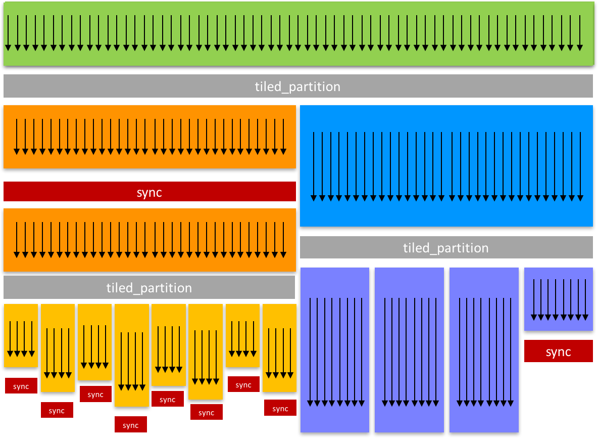
The above figure illustrates cooperative groups (source: https://devblogs.nvidia.com/cooperative-groups). The beginning (and ending) of a grid group essentially triggers a repartitioning of the threads.
Also useful to note is that {!end_grid_group} does not perform a grid synchronization, but can be seen as a “soft” separator which does not involve any memory or thread barrier. Together with a grid synchronization syncthreads grid, the grid group body will be applied to every element of the data (in this case membership[pos]).
To keep the programming simple, the Quasar compiler provides an elegant mechanism to automatically generate grid groups, through the use of designated shared memory. The above kernel function can written in a simpler way:
function [] = __kernel__ clustering_kernel(data:mat(:,3),centroids:mat(16,3),membership:vec[int],pos:int,blkpos:int,blkdim:int)
{!function_transform enable="sharedmempromotion"}
d=zeros(256)
for k=0..255
d[k]=sum(((centroids[k,0..2]-data[pos,0..2]).^2))
endfor
membership[pos]=argmin(-d)
endfunction By inserting the code attribute {!function_transform enable="sharedmempromotion"} and by explicitly indicating the dimensions of centroids the compiler recognizes that the variable centroids is best accessed from the shared memory of the GPU. The compiler recognizes that the caching needs to be performed the least number of times possible, therefore it will automatically generate a grid group.
Performance result:
| Configuration: | Execution time |
|---|---|
| With grid group+shared memory | 268.87 ms |
| Global memory | 1493.382 ms |
Example use case 1: K-Means
The following K-Means example illustrates some thorough compiler optimization, which causes:
- for-loops to be parallelized
- temporary results (like
d) to be stored in the GPU registers - the
centroidsandcountvariables to be cached in shared memory - use of grid groups to optimally reuse the cached data
- parallel reduction algorithm to compute
costfn - automatic kernel generation for the normalization operation at the end.
function [costfn] = kmeans_clustering_it[N:int,K:int](data : mat(:,N), centroids : mat(K,N), membership : vec[int])
M = size(data,0) % number of data samples
assert(numel(membership) == M, "membership vector has invalid length")
{!function_transform enable="sharedmempromotion"}
% update the membership
costfn = 0.0
{!parallel for}
for m=0..M-1
sample = data[m,:]
d = zeros(K) % dynamic kernel memory avoided by type parameter
% for each cluster
for k=0..K-1
d[k] = sum((centroids[k,:] - sample).^2)
endfor
membership[m] = index_of_max(-d)
costfn += min(d)
endfor
% update the cluster centers
count = zeros(K)
{!parallel for}
for k=0..M-1
mship = membership[k]
count[mship] += 1
centroids[mship,:] += data[k,:]
endfor
% normalization
centroids ./= repmat(transpose(max(1,count)),[1,N])
endfunctionTo enable these optimizations, in this case, it is required to have a generic kernel function with parameters N:int, K:int. This way, the dimensions of data and centroids are partially known at compile-time, which allows the compiler to calculate the amount of shared memory that is required. The compiler can choose the memory type (e.g., registers, shared memory, global memory) depending on the dimensions of the data. Of course, this can also be controlled programatically:
| Memory type | Required technique |
|---|---|
| Registers | Use fixed-sized data types, do not enable sharedmempromotion |
| Shared memory | Use fixed-sized data types, enable sharedmempromotion |
| Global memory | Pass vec, mat, cube type without dimensions specified |
| Constant memory | Use 'hwconst modifier (Kernel parameters only) |
Example use case 2: Single-kernel Parallel Sort
In this Section, we implement a parallel bitonic sort algorithm that takes maximally advantage of shared memory and that only launches a single megakernel. The megakernel replaces smaller kernels that would otherwise have been launched successively, thereby reducing the kernel launch overhead. To achieve this, we use grid groups as well as grid synchronization: syncthreads grid (which places a barrier for all threads within the grid). This is in contrast with syncthreads block (which places a barrier for only the threads within the current block).
The following function sorts all rows of a matrix (with generic element type):
function [] = fast_sort[T](x : mat[T])
function [] = __kernel__ bitsort(s : mat[T]'unchecked, x : mat[T]'unchecked, _
log2_n : int, pos : ivec2)
% Load data in shared memory with the specified stride
B : int'const = 1024
s_sh : vec[T]'unchecked = shared[T](B)
{!cuda_launch_bounds max_threads_per_block=1024}
{!begin_grid_group}
% Read input
s[pos] = pos[1] < size(x,1) ? x[pos] : maxvalue(T)
syncthreads grid
for k=1..log2_n % Outer loop
for log2j_base = k-1..-9..0 % -9 = log2_cols = log2(B)-1
log2j_end = max(0, log2j_base-8)
{!begin_grid_group}
% Rotate (log2_n-log2j_end) bits right
src_index = shl(and(pos[1],shl(1,log2_n-log2j_end)-1),log2j_end) + _
shr(pos[1],log2_n-log2j_end)
i = and(pos[1], B-1)
b = and(src_index, shl(1, k))>0
s_sh[i] = s[pos[0], src_index]
syncthreads block
for log2j=log2j_base-log2j_end..-1..0
ixj = xor(i, shl(1,log2j))
if i < ixj
v = (ixj - i) * b + i
w = (i - ixj) * b + ixj
if s_sh[v] > s_sh[w]
tmp = s_sh[v]; s_sh[v] = s_sh[w]; s_sh[w] = tmp
endif
endif
syncthreads block
endfor
s[pos[0], src_index] = s_sh[i]
syncthreads grid
{!end_grid_group}
endfor
endfor
syncthreads grid
% Write output
if pos[1] < size(x,1)
x[pos] = s[pos]
endif
{!end_grid_group}
endfunction
n = max(1024,nextpow2(size(x,1))) % bitonic sort only handles
% powers of two, so we perform padding (only in our temporary buffer)
s = uninit[T](size(x,0), n)
parallel_do([[size(x,0),n,1],[1,1024,1]],s,x,round(log2(n)),bitsort)
endfunctionNote that {!begin_grid_group}...{!end_grid_group} is used two times, in a nested way. The outer grid group is used to separate the shared memory allocation from the other operations, causing the shared memory allocations to be performed sparingly. The inner grid group constitutes an inner parallel region, it would be the same as calling parallel_do(..., inner_kernel), but this avoids calling a kernel function. In fact, cooperative groups enable repartitioning the work amongst the threads.
Cooperative threading
Every year, GPU programming becomes more feature rich. Accordingly, it is time to update the thread synchronization and inter-thread communication primitives of Quasar. Below is a preliminary overview.
Synchronization granularity
The keyword syncthreads now accepts a parameter that indicates which threads are being synchronized. This allows more fine grain control on the synchronization.
| Keyword | Description |
|---|---|
syncthreads(warp) |
performs synchronization across the current (possibly diverged) warp (32 threads) |
syncthreads(block) |
performs synchronization across the current block |
syncthreads(grid) |
performs synchronization across the entire grid |
syncthreads(multi_grid) |
performs synchronization across the entire multi-grid (multi-GPU) |
syncthreads(host) |
synchronizes all host (CPU and GPU threads) |
The first statement syncthreads(warp) allows divergent threads to synchronize at any time (it is also useful in the context of Volta’s independent scheduling). syncthreads(block) is equivalent to syncthreads in previous versions of Quasar. The grid synchronization primitive syncthreads(grid) is particularly interesting, it is a feature of CUDA 9 that was not available before. It allows to place barriers inside kernel function that synchronize all blocks. The following function:
function y = gaussian_filter_separable(x, fc, n)
function [] = __kernel__ gaussian_filter_hor(x : cube, y : cube, fc : vec, n : int, pos : vec3)
sum = 0.
for i=0..numel(fc)-1
sum = sum + x[pos + [0,i-n,0]] * fc[i]
endfor
y[pos] = sum
endfunction
function [] = __kernel__ gaussian_filter_ver(x : cube, y : cube, fc : vec, n : int, pos : vec3)
sum = 0.
for i=0..numel(fc)-1
sum = sum + x[pos + [i-n,0,0]] * fc[i]
endfor
y[pos] = sum
endfunction
z = uninit(size(x))
y = uninit(size(x))
parallel_do (size(y), x, z, fc, n, gaussian_filter_hor)
parallel_do (size(y), z, y, fc, n, gaussian_filter_ver)
endfunctionCan now be simplified to:
function y = gaussian_filter_separable(x, fc, n)
function [] = __kernel__ gaussian_filter_separable(x : cube, y : cube, z : cube, fc : vec, n : int, pos : vec3)
sum = 0.
for i=0..numel(fc)-1
sum = sum + x[pos + [0,i-n,0]] * fc[i]
endfor
z[pos] = sum
syncthreads(grid)
sum = 0.
for i=0..numel(fc)-1
sum = sum + z[pos + [i-n,0,0]] * fc[i]
endfor
y[pos] = sum
endfunction
z = uninit(size(x))
y = uninit(size(x))
parallel_do (size(y), x, y, z, fc, n, gaussian_filter_separable)
endfunctionThe advantage is not only in the improved readability of the code, but the number of kernel function calls can be reduced which further increases the performance. Note: according to the NVidia documentation this feature will require at least a Pascal GPU.
On the other hand, it is possible to launch a kernel over multiple GPUs using a new function multi_parallel_do. This requires 1) a Pascal type GPU and 2) the GPUs to be identical.
Interwarp communication
Special kernel function parameters (similar to blkpos, pos etc.) are added to control the GPU threads.
| Parameter | Type | Description |
|---|---|---|
coalesced_threads |
thread_block |
a thread block of coalesced threads |
this_thread_block |
thread_block |
describes the current thread block |
this_grid |
thread_block |
describes the current grid |
this_multi_grid |
thread_block |
describes the current multi-GPU grid |
The thread_block class has the following properties:
| Property | Description |
|---|---|
thread_idx |
Gives the index of the current thread within a thread block |
size |
Indicates the size (number of threads) of the thread block |
active_mask |
Gives the mask of the threads that are currently active |
The thread_block class has the following methods:
| Method | Description |
|---|---|
sync() |
Synchronizes all threads within the thread block |
partition(size : int) |
Allows partitioning a thread block into smaller blocks |
shfl(var, src_thread_idx : int) |
Direct copy from another thread |
shfl_up(var, delta : int) |
Direct copy from another thread, with index specified relatively |
shfl_down(var, delta : int) |
Direct copy from another thread, with index specified relatively |
shfl_xor(var, mask : int) |
Direct copy from another thread, with index specified by a XOR relative to the current thread index |
all(predicate) |
Returns true if the predicate for all threads within the thread block evaluates to non-zero |
any(predicate) |
Returns true if the predicate for any thread within the thread block evaluates to non-zero |
ballot(predicate) |
Evaluates the predicate for all threads within the thread block and returns a mask where every bit corresponds to one predicate from one thread |
match_any(value) |
Returns a mask of all threads that have the same value |
match_all(value) |
Returns a mask only if all threads that share the same value, otherwise returns 0. |
In principle, the above functions allow threads to communicate with each other, without relying on, e.g., shared memory. The shuffle operations allow taking values from other active threads (active means not disabled due to thread divergence). all, any, ballot, match_any and match_all allow to determine whether the threads have reached a given state.
The warp shuffle operations require a Kepler GPU and allow the use of shared memory to be avoided (register access is faster than shared memory). This may bring again performance benefits for computationally intensive kernels such as convolutions and parallel reductions (sum, min, max, prod etc.).
Using this functionality will require the CUDA target to be specified explicitly (i.e., the functionality cannot be easily simulated by the CPU). This may be obtained by placing the following code attribute inside the kernel: {!kernel target="nvidia_cuda"}. For CPU execution a separate kernel needs to be written. Luckily, several of the warp shuffling optimizations can be integrated in the compiler optimization stages, so that only one single kernel needs to be written.
Example: parallel reduction using warp-shuffling operations
Cooperative groups using warp-shuffling operations can be used to implement a parallel reduction. The advantage of this approach is that the sum of the elements of the vector can be calculated without using shared memory. Note that the code below assumes that the warp size is 32. It is possible to use a for-loop instead, however, this degrades the performance somewhat. Because coalesced_threads are only supported by the CUDA backend, it is also required to set the code attribute {!kernel target="nvidia_cuda"}.
function y : scalar = __kernel__ reduce_sum(coalesced_threads : thread_block, x : vec'unchecked, blkpos : int, pos : int, blkdim : int, blkcnt : int)
{!kernel target="nvidia_cuda"}
lane = coalesced_threads.thread_idx
total = 0.0
for index=pos..blkdim*blkcnt..numel(x)-1
val = x[index]
val += coalesced_threads.shfl_down(val, 16)
val += coalesced_threads.shfl_down(val, 8)
val += coalesced_threads.shfl_down(val, 4)
val += coalesced_threads.shfl_down(val, 2)
val += coalesced_threads.shfl_down(val, 1)
total += val
endfor
% Atomics for accumulatino
if lane==0
y += total
endif
endfunctionIn general is beneficial when: * Shared memory is already used by the kernel for other purposes (e.g., caching other variables) * When the data to be aggregated does not fit in the shared memory * To maximize the occupancy by reducing shared memory pressure.
Remark: due to the atomic operation +=, the result is not deterministic: floating point rounding errors depend on the order of the operations. For an atomic add, the order of operations is not specified. This can be solved by storing the intermediate results in a vector, and summing this vector independently. # Code Workbench Tutorial
The code workbench window allows you to browse the code generated by the Quasar compiler. In fact, starting from the original source code you can visualize how every function (either host, kernel or device function) is processed. Moreover, the tool allows you to interactively apply and test compiler optimizations.
The code workbench window can be activated from the main menu (View/tool windows/Code workbench) or by pressing the F6 key. A screenshot is given below:
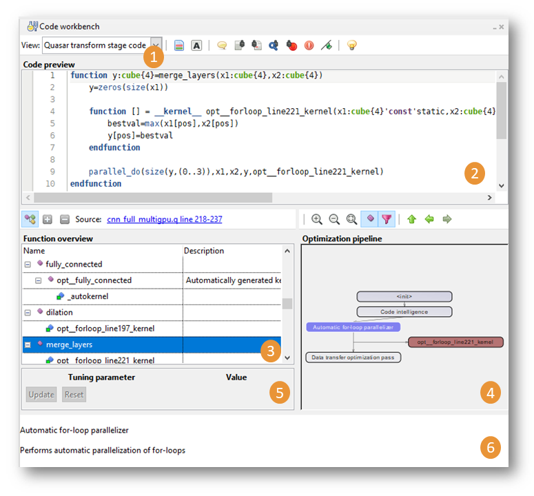
Once activated, the code workbench window will automatically update its content depending on the cursor location in the source code editor. When you select a certain function, the window will also jump to this function. The code workbench window consists of:
View selection:
Different view selection options are available:
View selection Description Quasar transform stage code Inspect the intermediate code generated during the various compilation stages Quasar final intermediate code Inspect the final intermediate code (e.g. during debugging) C++ code View the C++ code generated by the C++ backend CUDA code View the CUDA code generated by the CUDA backend OpenCL code View the OpenCL code generated by the OpenCL backend NVIDIA CUDA PTX code View PTX code resulting from compiling the CUDA code (NVIDIA CUDA compiler) NVIDIA OpenCL PTX code View PTX code resulting from compiling the CUDA code (NVIDIA OpenCL compiler) The Quasar transform stage code is mostly useful to investigate the optimizations applied to the source code (see point 4).
Code preview: displays source code/intermediate code. The textbox is read-only and cannot be changed. Note that as the source code is rendered from an intermediate representation, whitespaces and commands have been lost in the representation. Instead the code is nicely layout and indented.
Function overview: displays all functions present in the current Quasar module. The functions are shown hierarchically in the order defined in the source code file. Note that also auto-generated functions are displayed here. These functions have prefix
opt__. The description column gives the reason why this function was generated.Optimization pipeline: displays an optimization graph with the optimizations that were performed to the Quasar module (as source-to-source transformations). Only optimizations are shown that are applicable. To see the code changes, click on individual nodes of the optimization pipeline. It is possible to have a KDiff-like difference view on the code changes, by clicking onto the “red-green file” icon in the main toolbar of the code workbench window.
In brown, automatically generated functions are displayed. When double-clicking, the code workbench will jump to the selected function.
It may occur that the optimization pipeline splits into two branches, like in the following example:
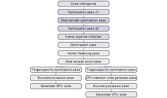
Optimization pipeline Here, the left branch represents the generated CPU-specific code, while the right branch contains the generated GPU-specific code. Because the Quasar compiler performs target-specific optimizations, the code generated for multiple platforms generally differs.
Tuning parameter window: some optimizations are not done automatically, because they might affect the performance in a positive way (but also in a negative way). By viewing and altering the tuning parameters in this window, the user can check some opportunities for further optimization. When the value of a tuning parameter is changed, it is necessary to click the Update button. This will insert the following code attribute to the original source code
{!tuning_param name="$param_imperfectloop"; range=[false,true]; default=true; desc="Line 242-263 - Parallelization preprocessing step for imperfect loops"}The compiler will then immediately apply the enabled optimization and the result can be inspected again in the code workbench window.
Help window: displays extra information in a context-sensitive way. For example, a short explanation of a
Debugging Type Inference results
When switching the code workbench window to the “Quasar final intermediate code” view, it is possible to inspect the type information associated to the intermediate code, by just hovering with the mouse over the functions/variables. This allows tracking down type-related issues in the code.
Debugging Automatically Generated Code
The code workbench window also offers the ability to debug automatically generated code. When debugging code and the program breaks (for example by pushing the break button, or due to an error), the current debugging location is displayed in the code workbench window:
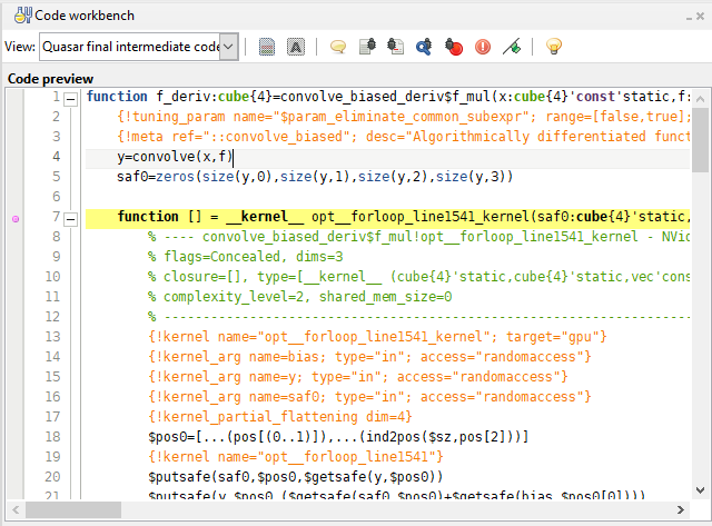
The call stack typically displays both user defined and automatically generated functions:
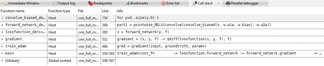
when double-clicking onto an automatically generated function, the code workbench window will navigate to the generated code. Stepping the program will update both the debug location in the source code editor as well as in the code workbench window. This makes it convenient to investigate errors that occur in automatically generated code.
Conclusion
The code workbench window gives insight on optimizations done under the hood, allows to check intermediate code generated during the various optimization stages, offers an interactive environment for setting and adjusting tuning parameters and for debugging.