Title: Quasar - CUDA Support GUIDE

Preface

This document contains information on the CUDA features that are currently supported in Quasar, how they can be accessed and used from within Quasar.

The goal is to make a wide set of CUDA features available to a user group that has no (or limited) experience with programming in CUDA, or to teams that do not have the available time resources available to do low-level CUDA programming.

The CUDA back-ends in Quasar closely follow the features new CUDA releases so that 1) the specific performance improving CUDA features are accessible from Quasar and so that 2) the end-users can benefit from buying new NVidia GPUs. The final goal is that when switching to newer GPUs, they see an acceleration of their algorithms, without having to do any efforts or changing their programs.

Roughly speaking, we can distinguish the CUDA features in two classes:

CUDA features that are used automatically by Quasar. Examples are: shared memory, CUFFT, dynamic parallelism, OpenGL interoperability, CUDA streams and synchronization, stream callbacks…
CUDA features in which the user has to make small modifications to the program in order to see the effects. Examples are: the use of hardware texturing units, the use of 16-bit floating point formats, the use of the non-coherent constant cache…

Some features impact the code generation, while other features impact the run-time. Because host/kernel and device functions are all described from within Quasar, the Quasar compiler has a good view on the intentions of the programmer and can take appropriate action (e.g., applying various code transformations, or adding meta information that may help the run-time).

This document also discusses several techniques that are currently available in the Quasar compiler/run-time.

CUDA features

Running kernels on the GPU

A simple example of a kernel that can be executed on the GPU is given below:

im = imread("image.png")
im_out = zeros(size(im))

function [] = __kernel__ filter_kernel(x, y : 'unchecked, mask, dir, pos)
    offset = int(numel(mask)/2)
    total = 0.
    for k=0..numel(a)-1
        total += x[pos + (k - offset).* dir] * mask[k]
    endfor
    y[pos] = total
endfunction

parallel_do(size(im),im,im_out,[1, 2, 3, 2, 1] / 9,[0,1],filter_kernel)

First, the kernel function filter_kernel is defined. Then, an image is read from the hard disk (imread). Next, the output image is allocated an initialized with zeros (zeros). Finally, the parallel_do function runs the kernel filter_kernel, which filters the image using the specified filter mask [1,2,3,2,1]/9.

Kernel functions need to be declared using the __kernel__ modifier. Although, technically, this modifier could even be omitted from the Quasar language specification, it brings transparency to the user about which functions eventually will be executed on the GPU device.

When running kernel functions, the run-time system automatically adapts the block dimensions, shared memory size, to the GPU parameters obtained using the CUDA run-time API. The run-time also makes sure that the data dimensions are a multiple of the block dimensions, thereby maximizing the occupancy of the resulting kernel. If necessary, the run-time system will run a version of the kernel that can process data dimensions that are not a multiple of the block dimensions.

Depending on the characteristics of the kernel (determined at compile-time), the run-time system also chooses the cache configuration of the kernel: to trade-off shared memory vs. data caching.

To define kernels in Quasar, lambda expressions can also be used, if that is more convenient. In combination with (automatic) closure variables, we can define the above filter simply as:

parallel_do(size(im),__kernel__ (pos) -> y[pos] =
    (x[pos+[0,-2]]+x[pos[0,2]]+2*(x[pos+[0,-1]]+x[pos+[0,1]]+3*x[pos])/9)

Note that in this example, the filter mask [1,2,3,2,1]/9 is substituted in the kernel function, which is a manual optimization. However, the compiler is able to do this optimization automatically. Even in the first example, the variables dir and mask are determined to be constants by the compiler, and a specialization of the kernel filter_kernel is generated automatically that utilizes this constantness.

Alternatively, in many cases, kernel functions may be generated automatically by the Quasar compiler. For example, for matrix expressions A+B.*C+D[:,:,2] the compiler may generate a kernel function. Idem for the automatic loop parallelizer. Consider the loop:

x = imread("image.png")
y = zeros(size(x))
for m=0..size(y,0)-1
    for n=0..size(y,1)-1
        for k=0..size(y,2)-1
            y[m,n,k] = (x[m,n-2,k]+x[m,n+2,k] + 2*(x[m,n-1,k]+x[m,n+1,k])+3*x[m,n,k])/9
        endfor
    endfor
endfor

For the above loop, the compiler will perform a dependency analysis and determine that the loop is parallelizable. Subsequently, a kernel function and parallel_do call will automatically be generated. This relieves the user from thinking in terms of kernel functions and parallel loops.

Device functions

To enable kernel functions to share functionally, __device__ functions can be defined. __device__ functions can be called from either host functions (i.e. without __kernel__/__device__) or other kernel/device functions. An example is given below:

function y = __device__ hsv2rgb (c : vec3)
    h = int(c[0] * 6.0)
    f = frac(c[0] * 6.0)
    v = 255.0 * c[2]    
    p = v * (1 - c[1])
    q = v * (1 - f * c[1])
    t = v * (1 - (1 - f) * c[1])
    match h with
    | 0 -> y = [v, t, p]
    | 1 -> y = [q, v, p]
    | 2 -> y = [p, v, t]
    | 3 -> y = [p, q, v]
    | 4 -> y = [t, p, v]
    | _ -> y = [v, p, q]
    endmatch
endfunction

Note the compact syntax notation in which vectors can be handled.

Device functions can be generic (like template functions in C++). In Quasar, it suffices to not specify any type of the function arguments. The following lambda expression

norm = __device__ (x) -> sqrt(sum(x.^2))

will then be specialized for every usage. For example, one can call the function with a scalar number (norm(-2)=2) or using a vector (norm([3,4])=5).

Block position, block dimensions, block index

Several GPU working parameters can be accessed via special kernel function parameters (with a fixed name). For example:

function [] = __kernel__ traverse(pos, blkpos, blkdim, blkidx)
   ...
endfunction

The meaning of the special kernel function parameters is as follows:

Parameter name	Meaning
pos	Position
blkpos	Position within the current block
blkdim	Block dimensions
blkidx	Block index
blkcnt	Block count (grid dimensions)
warpsize	Size of a warp

Correspondingly, the pos argument is calculated (internally) as follows:

pos = blkidx .* blkdim + blkpos

The type of the parameters can either be specified by the user (e.g., ivec2: an integer vector of length 2), or determined automatically through type inference.

By default, the block dimensions are determined automatically by the Quasar runtime system, but optionally, the user can specify the block dimensions manually, using the parallel_do function.

The maximum block size for a given kernel function can be requested using the function max_block_size. An optimal block size can be calculated with the function opt_block_size.

Datatypes and working precision

Quasar supports both integer, scalar (floating point) and complex scalar data data types. Typically, the global floating point working precision is specified at a global level (inside the Quasar Redshift IDE). This allows the user to change the precision of his program at any point, which allows him/her to investigate the accuracy or performance benefits of a different working precision. Two precision modes are supported (single precision and double precision) in global mode. The impact of the working precision is global, and leads to different sets of functions to be called internally. For example, cuFFT can be used in single or in double precision mode; this is done automatically (the user does not need to change the code, as it suffices to call the fft1, fft2 or fft3 functions).

In case mixed floating point precision are indended, it is also possible to explicitly allocate matrices with a specified precision. Three precision modes are supported (half, single, double precision):

    A_half = typename(mat[scalar'half])(100,100)
    A_single = typename(mat[scalar'single])(100,100)
    A_double = typename(mat[scalar'double])(100,100)

Note that Quasar’s runtime by default only support functions in the global precision. Import floattypes.q to use functions on non-global precision types (for example half).

For maximal performance, kernels involving half precision floating point numbers are best vectorized to use the 32-bit vec[scalar'half](2) SIMD type. See below in the SIMD section.

Atomic operations

Atomic operations have a special syntax in Quasar. Whenever a compound assignment operator is used (e.g., +=,-=,…) on a vector/matrix variable that is stored in the global/shared memory of the GPU, an atomic operation is performed. Atomic operations are supported for integers and floating point numbers. The following table lists the types of supported atomic operations.

Operator	Meaning
+=	Atomic add
-=	Atomic subtract
*=	Atomic multiply
/=	Atomic divide
^=	Atomic power
.*=	Atomic pointwise multiplication (e.g. for vectors)
./=	Atomic pointwise division (e.g. for vectors)
.^=	Atomic pointwise power (e.g. for vectors)
&=	Atomic bitwise AND
\|=	Atomic bitwise OR
~=	Atomic bitwise XOR
^^=	Atomic maximum
__=	Atomic minimum

The result of the atomic operation is the value obtained after the operation. For example, for a=0; b=(a+=1), we will have that b=1.

The use of atomic operations is very convenient, especially for writing functions that aggregate the data, like:

x = imread("image.tif")
[sum1,sum2] = [0.0,0.0]
for m=0..size(x,0)-1
    for n=0..size(x,1)-1
        sum1 += x[m,n]
        sum2 += x[m,n]^2
    endfor
endfor

A direct translation to atomic operations on the GPU does not lead to the most optimal performance (because the operations will be serialized internally). Therefore, to be able to benefit from the simplicity in implementing summing/other aggregation algorithms, the Quasar compiler automatically recognizes aggregation variables, and translates the resulting loop to a more efficient parallel sum reduction algorithm using shared memory. This often improves the performance by a factor of ten!

Atomic exchange, compare and exchange

Some parallel algorithms rely on atomic exchange / compare and exchange operations. These operations can be implemented using the <- operator.

Atomic exchange:

old_val = (a[0] <- new_val)

Atomic compare and exchange:

old_val = (a[0] <- (expected_val, new_val))

The above atomic operations can be used to implement concurrent data structures, mutexes and semaphores. Note however that the GPU hardware may execute CUDA warps in a lock-step, causing deadlocks when atomic compare and exchange operations are used. Also for performance reasons it is recommended to avoid intensive reliance on atomic (compare and) exchange operations.

It seems that - inspite of being used intensively on the CPU - these operations can often be avoided by using simpler synchronization mechanisms provided by the GPU (e.g., shared memory, thread synchronization, warp shuffling, …).

Shared memory and thread synchronization

As mentioned in the previous section, the compiler may generate code that uses the shared memory of the GPU automatically. In fact, the compiler is able to detect certain programming patterns and to replace them by algorithms that make use of shared memory. Some examples are:

Stencil operations (e.g., convolution)
Parallel reduction algorithms
Parallel prefix sum algoritms
Histogram computations (see documentation on shared memory designators)

This alleviates the user from writting algorithms making use of the shared memory. However, in some cases, it is also useful to manually write algorithms that store intermediate values in the shared memory. Therefore, shared memory can be allocated using the function shared (or optionally using shared_zeros, in case the memory needs to be initialized with zeros). Thread synchronization is performed using the keyword syncthreads. An example is given below:

function y = gaussian_filter(x, fc, n)
    function [] = __kernel__ kernel(x:cube,y:cube'unchecked,fc:vec'unchecked'hw_const,n:int,pos:ivec3,blkpos:ivec3,blkdim:ivec3)        
        [M,N,P] = blkdim+[numel(fc),0,0]
        assert(M*N*P<=1024)  % put an upper bound on the amount of shared memory
        vals = shared(M,N,P) % allocate shared memory

        sum = 0.
        for i=0..numel(fc)-1   % step 1 - horizontal filter
            sum += x[pos[0]-n,pos[1]+i-n,blkpos[2]] * fc[i]
        endfor
        vals[blkpos] = sum  % store the result

        if blkpos[0]<numel(fc) % filter two extra rows (needed for vertical filtering
            sum = 0.
            for i=0..numel(fc)-1
                sum += x[pos[0]+blkdim[0]-n,pos[1]+i-n,blkpos[2]] * fc[i]
            endfor
            vals[blkpos+[blkdim[0],0,0]] = sum
        endif

        syncthreads(block)  % thread synchronization for the current block

        sum = 0.
        for i=0..numel(fc)-1   % step 2 - vertical filter
            sum += vals[blkpos[0]+i,blkpos[1],blkpos[2]] * fc[i]
        endfor
        y[pos] = sum
    endfunction
    y = uninit(size(x))
    parallel_do (size(y), x, y, fc, n, kernel)
endfunction

Here, it is worth mentioning that the assertion M*N*P<=1024 helps the compiler, to determine an upper bound for the amount of shared memory that needs to be reserved for the kernel function. This allows for multiple blocks to be processed in parallel on the GPU (maximizing the occupancy).

As an alternative, shared memory designators have been added to Quasar. A variable can explicitly be annotated to be stored in shared memory, using the 'shared accessor. The Quasar compiler then generates the necessary code to transfer the data to shared memory and to distribute the copy task/calculations over the different threads. This significantly simplifies the code and improves the readability.

function [] = __kernel__ kernel(A : mat, a : scalar, b : scalar, pos : ivec3)

    B : 'shared = transpose(a*A[0..9, 0..9]+b) % fetch
    % ... calculations using B (e.g., directly with the indices)
    A[0..9, 0..9] = transpose(B) % store

endfunction

Thread synchronization

The keyword syncthreads accepts a parameter that indicates which threads are being synchronized. This allows more fine grain control on the synchronization.

Keyword	Description
`syncthreads(warp)`	performs synchronization across the current (possibly diverged) warp (32 threads)
`syncthreads(block)`	performs synchronization across the current block
`syncthreads(grid)`	performs synchronization across the entire grid
`syncthreads(multi_grid)`	performs synchronization across the entire multi-grid (multi-GPU)
`syncthreads(host)`	synchronizes all host (CPU and GPU threads)
`syncthreads`	alias for `syncthreads(block)`

The first statement syncthreads(warp) allows divergent threads to synchronize at any time (it is also useful in the context of Volta’s independent scheduling). syncthreads(block) is equivalent to syncthreads in previous versions of Quasar. The grid synchronization primitive syncthreads(grid) allows to place barriers inside kernel function that synchronize all blocks. The following example shows how to apply a separable filter to an input image.

function y = gaussian_filter_separable(x, fc, n)
    function [] = __kernel__ gaussian_filter_separable(x : cube, y : cube, z : cube, fc : vec, n : int, pos : vec3)
        sum = 0.
        for i=0..numel(fc)-1
            sum = sum + x[pos + [0,i-n,0]] * fc[i]
        endfor
        z[pos] = sum
        syncthreads(grid)
        sum = 0.
        for i=0..numel(fc)-1
            sum = sum + z[pos + [i-n,0,0]] * fc[i]
        endfor
        y[pos] = sum
    endfunction
    z = uninit(size(x))
    y = uninit(size(x))
    parallel_do (size(y), x, y, z, fc, n, gaussian_filter_separable)
endfunction

The advantage is not only in the improved readability of the code, but the number of kernel function calls can be reduced which further increases the performance. This feature also opens up the way to kernel fusion (see further), which intensively uses grid-level synchronization.

There are a few caveats with grid-level synchronization:

The number of active blocks should be less or equal than the total number of blocks that the GPU can process in parallel. This is to ensure that all active blocks can reach the grid barrier at the same time.
The values of locally declared variables (such as sum in the above example) are not preserved across grid barriers and need to be reinitialized.

The Quasar compiler enforces these conditions automatically. However, in case manual control of the block size and/or block count is desirable, the function opt_block_cnt needs to be used. This can be done as follows:

block_size = opt_block_size(kernel,data_dims)
grid_size = opt_block_cnt(kernel,block_size,data_dims)
parallel_do([grid_size.*block_size, block_size], kernel)

First, the optimal thread block size is calculated (which typically maximizes occupancy for a given kernel and data dimensions). Next, the grid size is optimized to ensure the grid-level synchronizations are satisfied.

Memory synchronization

The keyword memfence can be used to place memory barriers in the code; this is useful when threads need to wait for a global memory operation to be completed.

Keyword	Description
`memfence(grid)`	Suspends the current thread until its global memory writes are visible by all threads in the grid
`memfence(block)`	Suspends the current thread until its global memory writes are visible by all threads in the block
`memfence(system)`	Suspends the current thread until its global memory writes are visible by all threads in the system (i.e., CPU, GPU, …)

Cooperative groups

Kernels can have special arguments that give fine grain control over GPU threads

Parameter	Type	Description
`coalesced_threads`	`thread_block`	a thread block of coalesced threads
`this_thread_block`	`thread_block`	describes the current thread block
`this_grid`	`thread_block`	describes the current grid
`this_multi_grid`	`thread_block`	describes the current multi-GPU grid

The thread_block class has the following properties:

Property	Description
`thread_idx`	Gives the index of the current thread within a thread block
`size`	Indicates the size (number of threads) of the thread block
`active_mask`	Gives the mask of the threads that are currently active

The thread_block class has the following methods:

Method	Description
`sync()`	Synchronizes all threads within the thread block
`partition(size : int)`	Allows partitioning a thread block into smaller blocks
`shfl(var, src_thread_idx : int)`	Direct copy from another thread
`shfl_up(var, delta : int)`	Direct copy from another thread, with index specified relatively
`shfl_down(var, delta : int)`	Direct copy from another thread, with index specified relatively
`shfl_xor(var, mask : int)`	Direct copy from another thread, with index specified by a XOR relative to the current thread index
`all(predicate)`	Returns true if the predicate for all threads within the thread block evaluates to non-zero
`any(predicate)`	Returns true if the predicate for any thread within the thread block evaluates to non-zero
`ballot(predicate)`	Evaluates the predicate for all threads within the thread block and returns a mask where every bit corresponds to one predicate from one thread
`match_any(value)`	Returns a mask of all threads that have the same value
`match_all(value)`	Returns a mask only if all threads that share the same value, otherwise returns 0.

Warp shuffling operations

Cooperative groups using warp-shuffling operations can be used to implement a parallel reduction. The advantage of this approach is that the sum of the elements of the vector can be calculated without using shared memory. Note that the code below assumes that the warp size is 32. It is possible to use a for-loop instead, however, this degrades the performance somewhat. Because coalesced_threads are only supported by the CUDA backend, it is also required to set the code attribute {!kernel target="nvidia_cuda"}.

function y : scalar = __kernel__ reduce_sum(coalesced_threads : thread_block, x : vec'unchecked, blkpos : int, pos : int, blkdim : int, blkcnt : int)
    {!kernel target="nvidia_cuda"}
    lane = coalesced_threads.thread_idx
    total = 0.0

    for index=pos..blkdim*blkcnt..numel(x)-1    
        val = x[index]        
        val += coalesced_threads.shfl_down(val, 16)
        val += coalesced_threads.shfl_down(val, 8)
        val += coalesced_threads.shfl_down(val, 4)
        val += coalesced_threads.shfl_down(val, 2)
        val += coalesced_threads.shfl_down(val, 1)
        total += val
    endfor

    % Atomics for accumulation
    if lane==0
        y += total
    endif
endfunction

In general is beneficial when: * Shared memory is already used by the kernel for other purposes (e.g., caching other variables) * When the data to be aggregated does not fit in the shared memory * To maximize the occupancy by reducing shared memory pressure.

Remark: due to the atomic operation +=, the result is not deterministic: floating point rounding errors depend on the order of the operations. For an atomic add, the order of operations is not specified. This can be solved by storing the intermediate results in a vector, and summing this vector independently.

Warp shuffling operations can be even used to implement operations like convolutions. Below, we give an example of a Gaussian filter on an image:

function y = gaussian_filter_warpshuffle(x, fc, n)
    function [] = __kernel__ gaussian_filter[N:int](x : cube, y : cube'unchecked, z : cube, fc : vec'hwconst'unchecked, n : int, coalesced_threads : thread_block,  pos : vec3)
        {!kernel target="nvidia_cuda"}
        thread_idx = coalesced_threads.thread_idx
        x_warp = zeros(N)
        for i=0..N-1
            {!unroll}
            x_warp[i] = x[pos + [0, i * coalesced_threads.size, 0]]
        endfor
        syncthreads(warp)
        total = 0.0
        for i=0..n-1
            [k,l] = ind2pos([2, coalesced_threads.size], thread_idx+i)
            val = coalesced_threads.shfl(x_warp, l)
            total += val[k] * fc[i]
        endfor
        z[pos] = total % Intermediate result

        syncthreads(grid)
        % Shuffle pos
        blkpos = mod(pos, [32,32,1])
        pos2 = pos - blkpos + [blkpos[1], blkpos[0], 0]

        for i=0..N-1
            {!unroll}
            x_warp[i] = z[pos2 + [i * coalesced_threads.size, 0, 0]]
        endfor
        syncthreads(warp)
        total = 0.0
        for i=0..n-1
            [k,l] = ind2pos([2, coalesced_threads.size], thread_idx+i)
            val = coalesced_threads.shfl(x_warp, l)
            total += val[k] * fc[i]
        endfor
        y[pos2] = total
    endfunction
    y = uninit(size(x))
    z = uninit(size(y))
    parallel_do([size(y,0..2),[32,32,1]], x, y, z, fc, n, gaussian_filter[2])
endfunction

The idea is here to cache intensities of the input image in the registers. By using the warp shuffling operations, each thread can then access the cached intensity of another thread. Note that warp and grid synchronization are required in this particular implementation. The above code assumes that N = ceil((warp_size-1+numel(fc))/warp_size).

Memory optimizations

To optimize memory transfer and access, the Quasar compiler/run-time employ a variety of techniques, many of them relying on underlying CUDA features.

When a kernel function is started (using the parallel_do function), it is made sure that all kernel function arguments are copied to the GPU, and that the arguments are up to date. This is the automatic memory management function, that is performed by the Quasar run-time. The automatic memory management works the best with large blocks of memory. Therefore, in case of small structures, such as nodes of a linked lists, several connected structures are grouped in a graph and the graph is transferred at once to the device. However, in some cases it is useful to perform some extra memory optimizations.

Modifiers ’const and ’nocopy

The types of kernel function parameters can have the special modifiers 'const and 'nocopy. These modifiers are added automatically by the compiler after analyzing the kernel function. The meaning of this modifiers is as follows:

Type modifier	Meaning
`'const`	The vector/matrix variable is constant and only being written to
`'nocopy`	The vector/matrix variable does not need to be copied to the device before the kernel function is called

The advantage of these type modifiers is that it permits the run-time to avoid unnecessary memory copies

between host and the device
between devices (in multi-GPU processing modes)
between linear device memory and texture memory

In case of parameters with the 'const modifier, the dirty bit of the vector/matrix does not need to be set. For 'nocopy, it suffices to allocate data in device memory without initializing it.

Furthermore, the modifiers are exploited in later optimization and code generation passes, e.g. to take automatic advantage of caching capabilities of the GPU (see below).

An example of the modifiers is given below:

function [] __kernel__ copy_kernel(x:vec'const,y:vec'nocopy,pos:int)
    y[pos] = x[pos]
endfunction
x = ones(2^16)    
y = zeros(size(x))
parallel_do(numel(x),x,y,kernel)

Here 'nocopy is added because the entire content of the matrix y is overwritten.

Constant memory

NVIDIA GPUs typically provide 64KB of constant memory that is treaded differently from standard global memory. In some situations, using constant memory instead of global memory may reduce the memory bandwidth (which is beneficial for kernels). Constant memory is also most effective when all threads access the same value at the same time (i.e. the array index is not a function of the position). Kernel function parameters can be declared to reside in constant memory by adding the hw_const modifier:

function [] = __kernel__ kernel_hwconst(x : vec, y : vec, f : vec'hwconst, pos : int)
    sum = 0.0
    for i=0..numel(f)-1
        sum += x[pos+i] * f[i]
    endfor
    y[pos] = sum
endfunction

The use of constant memory may have a dramatic impact on the performance. In the above example, the computation time was improved by a factor 4x, by only adding 'hwconst modifier to the kernel function.

Texture memory

With the advent of CUDA, the GPU’s sophisticated texture memory can also be used for general-purpose computing. Although originally designed for OpenGL and DirectX rendering, texture memory has properties that make it very useful for computing purposes. Like constant memory, texture memory is cached on chip, so it may provide higher effective bandwidth than obtained when accessing the off-chip DRAM. In particular, texture caches are designed for memory access patterns exhibiting a great deal of spatial locality.

The Quasar run-time allocates texture memory (via CUDA arrays) and transparently copies data to the arrays when necessary. Texture memory has the advantage that it can efficiently be accessed using more irregular access patterns, due to the texture cache.

The layout of the CUDA array is generally different from the memory layout in global memory. For example, there is a global option that the user can choose to use 16-bit float textures (instead of the regular 32-bit float textures). This not only reduces the amount of texture memory but also offers performance enhancements due to the reduced memory bandwidths (e.g. for real-time video processing). When necessary, the Quasar run-time performs the necessary conversions.

In Quasar, it is possible to indicate that a vector/matrix needs to be stored as a hardware texture, using special type modifiers that can be used for kernel function argument types:

Type modifier	Meaning
`'hwtex_nearest`	Hardware textures with nearest neighbor interpolation
`'hwtex_linear`	Hardware textures with linear (1D), bilinear (2D) or trilinear (3D) interpolation

An example is the following interpolation kernel function:

function [] = __kernel__ interpolate_hwtex (y : mat, x : mat'hwtex_linear'clamped, scale : scalar, pos : ivec2)        
    y[pos] = x[scale * pos]
endfunction

Here, the type modifiers hwtex_linear and clamped are combined.

Note that in Quasar, several built-in type modifiers define what happens when data is accessed outside the array/matrix boundaries (as mat'hwtex_linear'clamped in the above example):

Type modifier	Meaning
`'unchecked`	No boundary checks are being performed
`'checked`	An error is generated when the array/matrix boundaries are exceeded
`'circular`	Access with circular extension
`'mirror`	Access with mirror extension
`'clamped`	Access with clamping
`'safe`	The array/matrix boundaries are extended with zeros

When using GPU hardware textures, the boundary conditions 'circular, 'mirror, 'clamped and 'safe are directly supported by the hardware, leading to an extra acceleration.

Additionally, multi-component hardware textures, can also be defined, using the following type modifiers:

Type modifier	Meaning
`'hwtex_nearest(n)`	Hardware textures with nearest neighbor interpolation, and `n` components
`'hwtex_linear(n)`	Hardware textures with linear (1D), bilinear (2D) or trilinear (3D) interpolation, and `n` components

The advantage is that complete RGBA-values can be loaded with only one texture lookup.

For devices with compute architecture 2.0 of higher, writes to hardware textures are also supported, via CUDA surface writes. This is done fully automatically and requires no changes to the Quasar code.

Correspondingly, a matrix can reside in (global) device memory, in texture memory, in CPU host memory, or even all of the above. The run-time system keeps track of the status bits of the variables.

Non-coherent Texture Cache

As an alternative for devices with compute capability 3.5 (or higher), the non-coherent texture (NCT) cache can be used. The NCT cache allows the data still be stored in the global memory, will utilizing the texture cache for load operations. This combines the advantages of the texture memory cache with the flexibility (ability to read/write) of the global memory.

In Quasar, kernel function parameters can be declared to be accessed via the NCT cache, by adding the modifiers 'hwtex_const. Internally, hwtex_const generates CUDA code with the __ldg() intrinsic.

Optionally, depending on the compiler settings, the compiler may also add hwtex_const modifiers automatically, when determined to be beneficial.

Host-pinnable memory

The memory transfer between CPU and GPU and vice versa is accelerated when page-locked host memory (PLH) is used. To take advantage of this acceleration, the Quasar runtime system will automatically allocate data in the PLH memory when needed. Note that PLH memory is even required in concurrent kernel execution mode (see below) in order for memory transfers to overlap with kernel executions.

The use of pinned host memory can be controlled using the runtime setting RUNTIME_CUDA_ENABLEPINNEDHOSTMEM.

Unified memory

CUDA unified memory is a feature introduced in CUDA 6.0. For unified memory, one single pointer is shared between CPU and GPU. The device driver and the hardware make sure that the data is migrated automatically between host and device. This facilitates the writing of CUDA code, since no longer pointers for both CPU and GPU need to be allocated and also because the memory is transferred automatically.

In Quasar, unified memory can be used by setting RUNTIME_CUDA_UNIFIEDMEMORYMODE to Always in Quasar.Runtime.Config.xml.

Streams and Concurrency

Quasar has two execution modes that can be specified by the user on a global level (typically from within the Quasar Redshift IDE):

non-turbo: perform only one kernel at the time (synchronous kernel execution)
turbo: overlap kernels/memory transfers when possible (asynchronous kernel execution)

The turbo execution mode is fully automatic and internally relies on the asynchronous CUDA API functions. In the background, dependencies between matrix variables, kernels etc. are being tracked and the individual memory copy operations and kernel calls are automatically dispatched to one of the available CUDA streams. This way, operations can be performed in parallel on the available GPU hardware. Often, the turbo mode enhances the performance by 10%-30%. Also, automatic multi-GPU processing can be obtained using this concurrency model (see further).

Moreover, in Quasar, the streaming mechanism is expanded to the CPUs, which allows configurations in which for example, 4 CPU streams (threads) are allocated, 2 GPUs with each 4 streams. A load balancer and scheduler will divide the workload over the different CPU and GPU streams. It is possible to configure the number of CPU streams and the number of GPU streams. For example, on an 8-core CPU, a two parallel loops may run concurrently each on 4 cores. Idem for a system with two GPUs, each GPU may have 4 streams and kernel functions can be scheduled to in total 8 streams.

For inter-device synchronization purposes (e.g., between CPU and GPU), stream callbacks (introduced in CUDA 5.0) are used automatically.

The run-time system can be configured to use host-pinnable memory by default. This the advantage that kernels can directly access memory on the CPU, but also in turbo mode, the asynchronous memory copy operations from GPU to the host are non-blocking.

Memory access pattern and computation optimizations

Kernel tiling

Kernel tiling is a kernel function code transformation that divides the data in blocks of a fixed size. There are three possible modes:

Global kernel tiling: the data is subdivided in blocks of, e.g., 32x32x1 or 32x16x1. All threads in the grid collaborate to first calculate the first block, then the second block, and so on. The loop that traverses all these blocks is placed inside the kernel function. Note that the blocks normally don’t corresponds to the GPU (CUDA) blocks. It is very common that a 1D block index traverses 2D or 3D blocks (also called grid-strided loop). Global kernel tiling has the following benefits:
- Threads are reused; the maximum number of GPU blocks can be reduced, saving thread initialization and destruction overhead
- Calculations independent of the block can be placed outside of the tiling loop
- Less dependency on the GPU block dimensions, resulting in more portable code
A disadvantages of global kernel tiling is that the resulting kernels are more complex and typically use more registers.

Global kernel tiling can be activated by placing one of the following code attributes in the kernel function: {!kernel_tiling dims=[32,16,1]; mode="global"; target="gpu"} {!kernel_tiling dims=auto; mode="global"; target="gpu"} The target (e.g., cpu, gpu) specifies for which platform the kernel tiling will be performed. It is possible to enable tiling for one platform but not for the other. By combining multiple code attributes it is also possible to specify different block sizes for different platforms. In case of automatic tiling dimensions, the runtime will search for suitable block dimensions that optimize the occupancy.

For certain kernels (e.g., involving parallel reduction, shared memory accumulation, …), global kernel tiling is performed automatically. Kernels that use grid-level synchronization primitives (without TCC driver mode cooperative grouping) are also automatically tiled globally. This is also required in order for kernel fusion (see lower) to work correctly.
Local kernel tiling: here, each thread performs the work of N consecutive work elements. Instead of having 1024 threads process a block of size 32x32, we have 256 threads processing the same block. Each thread then processes data in a single instruction multiple data (SIMD) fashion. Moreover, the resulting instructions can be even mapped onto SIMD instructions (e.g., CUDA SIMD/SSE/AVX/ARM Neon), if the hardware supports them. In the following example, a simple box filter is applied to a matrix with element type uint8. function [] = __kernel__ filter(im8 : mat[uint8], im_out : mat[uint8], K : int, pos : ivec(2)) [m,n] = pos r2 = vec[int](4) for x=0..K-1 r2 += im8[m,n+x+(0..3)] endfor im_out[m,n+(0..3)] = int(r2/(2*K)) endfunction Local kernel tiling can be activated by placing the following code attribute in the kernel function: {!kernel_tiling dims=[1,1,4]; mode="local"; target="gpu"} In case purely SIMD processing is intended, it is better to use the following code attribute (see below): {!kernel_transform enable="simdprocessing"} Advantages of local kernel tiling:
- Less threads, so less thread initialization and destruction overhead
- mapping onto SIMD possible (when the block dimensions are chosen according to the GPU platform).
- For some operations, recomputation of values can be avoided.
Disadvantages:
- The resulting kernels use more registers, which may negatively impact the performance in some cases (e.g. register limited kernels)
- Not all operations may be accelerated by hardware SIMD operations (for example, division operations).
- The compiler needs to ensure that the data dimensions are a multiple of the block size. If this is not the case, extra “cool down” code is added.
Hybrid tiling: combines the advantages of global and local kernel tiling. To activate hybrid tiling, code attributes for both local and global tiling can be placed inside the kernel function: {!kernel_tiling dims=auto; mode="global"; target="gpu"} {!kernel_tiling dims=[1,1,4]; mode="local"; target="gpu"} Hybrid kernel tiling usually occurs as a result of several compiler optimizations.

SIMD data types

CUDA vector instructions interact with 32-bit words. Depending on the precision (8-bit integer, 16-bit integer or 16-bit floating point), the vector length is either 2 or 4. The following SIMD datatypes are defined in floattypes.q and inttypes.h:

type i8vec4 : vec[int8](4)
type hvec2 : vec[scalar'half](2)

Floating point SIMD data types:

The half-precision floating point format (FP16) is useful to reduce the device memory bandwidth for algorithms which are not sensitive to the reduced precision. For half, only integers between -2048 and 2048 can exactly be represented. Integers larger than 65520 or smaller than -65520 are rounded toward respectively positive and negative infinity.

Next to the reduced bandwidth, starting with the Pascal architecture, the GPU also offers hardware support for computations using this type. To gain maximal performance benefits, it is best to use the 32-bit length 2 SIMD half type (hvec2). Use of hvec2 typically results in two numbers being calculated in parallel, leading to a performance that is similar to one single precision floating point (FP32) operation. However, a Volta or Turing GPU is required to obtain performance benefits from using calculation in half precision format. For Kepler, Maxwell and Pascal GPUs, hardware support for operations in half precision is notably slow, therefore it is best to use the half type only for storage purposes (i.e., calculations are performed in the single-precision floating point type).

The following table shows the operations that have been accelerated using half types. For unsupported operations, the computation will be performed in FP32 format, leading to extra conversions between FP32 and FP16.

Integer SIMD data types:

CUDA supports SIMD operations for 8-bit and 16-bit integer vectors that fit into a 32-bit words. Below is a table of the operations that are accelerated. For unsupported operations, the computation will be performed in 32-bit integer format, leading to extra conversions between 32-bit and 8/16-bit integer formats.

Automatic vectorization and SIMD processing:

Automatic vectorization can be enabled using:

{!kernel_transform enable="simdprocessing"}

The SIMD processing transform will automatically generate the kernel_tiling code attribute and will set the block dimensions based on the best suited SIMD width for the current platform. For half precision floating point types, the SIMD width is 2. For 8-bit integer types, the SIMD width is 4. The SIMD processing transform will identify read accesses and determine the best suitable SIMD width.

Memory coalescing transform

Memory coalescing means that when the threads in a block are accessing consecutive memory locations, all the accesses are combined into a single request (i.e., coalesced) by the GPU hardware. This however requires that kernels are written such that subsequent threads in a block access consecutive memory locations. For 1D kernels, this is often not a problem, but 2D, 3D kernels may not respect the memory coalescing condition.

When the data access pattern does not allow memory coalescing but a direct manipulation of the position vector pos does (e.g., via [pos[0],pos[2],pos[1]]), the Quasar compiler will perform this dimension permutation operation automatically.

By default, when using directly the position vector pos, Quasar launches kernels so that memory coalescing is always possible. The following code gives an example of a kernel that accesses [pos[1],pos[0]] rather than pos.

function [] = __kernel__ kernel(im : mat'unchecked, im_out : mat'unchecked, pos : ivec2)
        {!tuning_param name="$param_memcoalescing"; default=true}
        im_out[pos[1],pos[0]] = im[pos[1],pos[0]]
endfunction

parallel_do(size(im_out,[1,0]),im,im_out,kernel)

By setting {!tuning_param name="$param_memcoalescing"; default=true} the compiler will automatically correct the position vector and swap the elements of the size vector in the parallel_do call when needed.

Kernel fusion

Nowadays, it is not uncommon that a convolution operation on a Full HD color image takes around 10 microseconds. However, with execution times so low, for many GPU libraries this has the consequence that the bottleneck moves back from the GPU to the CPU: the CPU must ensure that the GPU is busy at all times. This turns out to be quite a challenge on its own: when invoking a kernel function, there is often a comined runtime and driver overhead in the order of 5-10 microseconds. That means that all launched kernel functions must provide sufficient workload. Because just a filtering operation on a Full HD image is already in the 5-10 microsecond range of execution time, many smaller parallel operations (e.g., operations with data dimensions< 512*1024) are often not suited anymore for the GPU, unless the computation is sufficiently complex. In the new features of CUDA 10 it is mentioned:

“The overhead of a kernel launch can be a significant fraction of the overall end-to-end execution time.”

CUDA 10 introduces a graph API, which allows kernel launches to be prerecorded in order to be played back many times later. This technique reduces CPU kernel launch cost, often leading to significant performance improvements. We notice however that CUDA graphs are a runtime technique; its compile-time equivalent is kernel fusion. In kernel fusion, several subsequent kernel launches are fused into one big kernel launch (called a megakernel). In older versions of CUDA, dependent kernels could not easily be fused, because every kernel execution imposes an implicit grid synchronization at the end of execution. This grid synchronization could only be avoided by using CUDA streams which allows independent kernels to be processed concurrently. More recently, grid barriers (which synchronizes “all threads” in the grid of a kernel function) have become available, either via cooperative groups (in CUDA 9) or via emulation techniques. These grid barriers open the way to kernel fusion of dependent kernels.

Obviously, any synchronization point such as a grid barrier involves a certain overhead, a time that GPU threads spend waiting for other threads to complete. The total overhead can be minimized by minimizing the number of synchronization points. On the other hand, grid barriers are entirely avoided when there are no dependencies between the kernels. This automatically means that reordering of kernel launches is an essential step of the automatic kernel fusion procedure.

The application of compile-time kernel fusion also has several other performance related benefits: when multiple kernels become one kernel often temporary data stored in global memory can be entirely moved to the GPU registers. Since accessing GPU registers is significantly faster than reading from/writing to global memory, the execution performance of kernels can be vastly improved. In addition, the compiler can reuse memory resources and eliminate memory allocations, essentially leading a static allocation scheme, in which all temporary buffers are preallocated, prior to launching the megakernel.

The kernel fusion also has a number of complicating factors: * It is neccessary to determine at compile-time that arrays (vectors, matrices, …) have the same size. Luckily, Quasar’s high level inference engine allows to achieve this. * Kernels are often launched with different data (i.e., grid and block) sizes, while launching a megakernel requires one size to be passed. In Quasar, this is achieved by performing automatic kernel tiling. * Kernels often operate on data of different dimensionalities (vector, matrix, …). In Quasar, this is solved by performing a kernel flattening transform in combination with a grid-strided loop.

The remedies for different data dimensions each involve a separate overhead, usually in the form of more registers used by the megakernel. This may lead to register-limited kernel launches, in which some GPU multiprocessors are underutilized because of insufficient register memory. Therefore, Quasar includes a dynamic programming based optimization algorithm that takes all these factors into account.

In short, kernel fusion in Quasar is achieved by placing:

{!kernel_fusion strategy="smart"}

inside the parent function of the kernel functions. Important to realize is that all functions called by this parent function are inlined, so that if the callees launch kernel functions on their own, these kernel fusions can also be fused into the mega kernel. The compiler therefore sees a sequence of kernel launches and has to determine 1) a suitable order to launch the kernels and 2) whether the kernels are suited to perform kernel fusion.

When performing kernel fusion, a strategy needs to be passed, which controls the cost function used by the optimization algorithm:

Kernel fusion strategy	Purpose
smart	Let the Quasar compiler decide what is the best strategy
noreordering	Performs kernel fusion, without reordering the kernel launches
minsyncgrid	Minimizes the number of required grid synchronization barriers
minworkingmemory	Minimizes the total amount of (global) memory required for executing the fused kernel
manual	Kernel fusion barriers placed in the code determine which kernels are fused

Kernel fusion barriers {!kernel_fusion barrier} may be added to prevent kernels from being fused. In this case, M kernels are fused into N kernels with 1 < N <= M.

Under some circumstances (which also depend on the kernel fusion strategy), the compiler may waive fusion of certain kernels. The reasons can be inspected in the kernel fusion code transform log, which is accessible through the code workbench window in Redshift.

CuFFT: CUDA FFT library

The CUDA fft library is natively supported using the functions fft1, fft2, fft3, ifft1, ifft2, ifft3 and real-valued versions real(ifft1(x)), real(ifft2(x)), real(ifft3(x)). Often, one is interested in the real part of the inverse Fourier transform. Via a reduction (which is defined in Quasar),

reduction x -> real(ifft3(x)) -> irealfft3(x)

all occurrences of real(ifft3(x)) will be converted to the real-valued version of the ifft3. Internally Quasar uses the CUDA FFT plan with C2R option for implementing real(ifft1(x)). When the input is real-valued, Quasar will use the R2C option. The CuFFT module also supports automatic streaming and multi-GPU processing (note however that Tesla Compute Cluster cooperative FFTs over multiple devices are currently not supported). For small data sizes, or on CPU target platforms, the FFTW library is used as a fallback.

The semantics of fft1 and fft2 slightly differ. fft1 applies an FFT along the last dimension (for example, the rows of a matrix) while fft2 performs a 2D FFT along the first and second dimension. All other dimensions are used as batch (when there are other non-singleton dimensions, a CUDA many FFT plan is created).

To explicitly specify along which dimensions the FFT should be applied, the fftn function can be used. For example, fftn(A : cube, [1, 2]) applies a 2D FFT along the second and third dimension. fftn can be used to perform 4D or 5D FFTs. The function internally uses combinations of 1D, 2D and 3D FFTs as only these FFTs are available in CuFFT. The function automatically handles all strides and determines the best suited batch dimensions. In some more complex situations, fftn may result in a sequence of FFTs.

CuFFT plan cache

To speed up subsequent FFT calls, Quasar uses a LRU cache to store FFT plans. FFT plans are allocated for fixed input dimensions. The first time that the fft function is called, the execution time may be much higher than other times, because the FFT plan is being constructed. Because each plan uses some amount of GPU memory, the number of plans that can be stored in the cache is limited. The value can be configured via the runtime setting RUNTIME_FFT_PLAN_MAXCACHESIZE.

CuDNN: CUDA Deep Neural Networks library

By importing "Quasar.DNN.dll", many functions of the cuDNN library can be accessed directly from Quasar.

The Quasar DNN uses the NCHW representation (4D) or NCDHW (5D) for tensors.

NCHW means that:

The first dimension represents the batches
The second dimension represents the channels/feature maps
The third dimension is the vertical image dimension
The fourth dimension is the horizontal image dimension

NCDHW means that:

The first dimension represents the batches
The second dimension represents the channels/feature maps
The third dimension is the depth image dimension
The fourth dimension is the vertical image dimension
The depth dimension is the horizontal image dimension

For convolution filters, possible representations of the filter mask are PCHW and PCDHW where C is the number of input channels/feature maps and where P is the number of output channels/feature maps.

This means that a cuDNN convolution filter performs a P x C matrix multiplication along the channels. The batches are processed individually. It is therefore possible to perform both 2D and 3D convolutions.

Structures:

qdnn_conv_descriptor: convolution descriptor for cuDNN

Property	purpose
`pad_w`	specifies the horizontal padding of the filter mask
`pad_h`	specifies the vertical padding of the filter mask
`pad_d`	specifies the depth padding of the filter mask
`u`	horizontal filter stride
`v`	vertical filter stride
`d`	depth filter stride
`dilation_w`	horizontal dilation factor
`dilation_h`	vertical filter stride
`dilation_d`	depth filter stride
`dims`	dimensionality of the convolution (4 or 5)
`fwd_algo`	specifies the forward convolution algorithm
`bwd_data_algo`	specifies the backward data convolution algorithm
`bwd_filter_algo`	specifies the backward filter convolution algorithm
`math_type`	specifies the hardware unit to use (default, tensorop)
`mode`	sets the convolution mode (convolution / crosscorrelation)

As padding values, typically half the size of the filter mask (width, height or depth) is used. The stride values allows upscaling the filter mask by inserting zeros. The dilation values allow the resulting image to be subsampled. Most commonly, the stride and upscaling factor is one.

In 4D, the convolution formula is as follows (using cross-correlation mode): \[y_{n,k,p,q} = \sum_c^C \sum_r^R \sum_s^S x_{n,c,p\cdot u+r \cdot \mathrm{dilation}_h,q\cdot v+s \cdot \mathrm{dilation}_w} w_{k,c,r,s}\]

In 5D the formula becomes (using cross-correlation mode): \[y_{n,k,o,p,q} = \sum_c^C \sum_t^T \sum_r^R \sum_s^S x_{n,c,o\cdot d + t\cdot \mathrm{dilation}_d, p\cdot u+r \cdot \mathrm{dilation}_h,q\cdot v+s \cdot \mathrm{dilation}_w} w_{k,c,t,r,s}\]

By setting mode="convolution" (default), the filter mask is flipped horizontally, vertically (and in depth).

Grouped convolutions can be enabled by setting “unconventional” values for the P and C parameters of the filter mask. The following grouped convolutions are currently supported:

Description	Input tensor	Filter tensor	Output tensor
Normal case	NxCxHxW	KxCxH’xW’	NxKxHxW
Grouped I	NxCxHxW	Kx1xH’xW’	NxKCxHxW
Grouped II	NxKCxHxW	1xKxH’xW’	NxCxHxW

Grouped I allows a convolution to be applied separately to every color channel, mapping C channels onto KC channels. Grouped II maps KC channels onto C channels, performing a Kx1 matrix multiplication within each group of K channels.

The following convolution algorithms are available:

Algorithm	Forward	Algorithm	Backward data	Backward filter
Auto	x	Auto	x	x
FFT	x	AlgoFFT	x	x
FFTwithtiling	x	N/A
GEMM	x	N/A
implicitGEMM	x	N/A
implicitprecompGEMM	x	N/A
winograd	x	winograd	x	x
N/A		Algo0	x	x
N/A		Algo1	x	x

qdnn_pooling_descriptor: pooling descriptor for cuDNN

Property	purpose
`pad_w`	specifies the horizontal padding of the pooling window
`pad_h`	specifies the vertical padding of the pooling window
`pad_d`	specifies the depth padding of the pooling window
`w`	width of the pooling window
`h`	height of the pooling window
`d`	depth of the pooling window
`stride_w`	horizontal pooling stride
`stride_h`	vertical pooling stride
`stride_d`	depth pooling stride
`mode`	sets the convolution mode (`Max` / `AverageCountIncludePadding` / `AverageCountExcludePadding`)
`maxpooling_nanopt`	sets the NaN propagation mode (`NotPropagateNan` / `PropagateNan`)

Note that when wrong parameter values are set, cuDNN may give a runtime error during the execution of the cudnn_convolution_* functions.

qdnn_activation_descriptor: activation descriptor for cuDNN

Property	purpose
`mode`	sets the activation mode (`Sigmoid`, `Relu`, `Tanh`, `ClippedRelu`, `Elu`, `Identity`)
`reluNaNOpt`	sets the NaN optimization method (`NotPropagateNan` / `PropagateNan`)
`reluCeiling`	clipping threshold to be used when the activation mode is ‘clippedrelu’

Functions:

Function	Description
`cudnn_activation_forward`	Calculates the gradient of the neural activation function
`cudnn_activation_backward`	Applies a pointwise neural activation function to the input signal
`cudnn_batchnormalization_forward_inference`	Calculates an inference step of the batch normalization algorithm
`cudnn_batchnormalization_forward_training`	Calculates a forward pass of the batch normalization algorithm
`cudnn_batchnormalization_backward`	Calculates a backpropagation step of the batch normalization algorithm
`cudnn_convolution_forward`	Calculates a forward convolution or cross-correlation using the cuDNN library
`cudnn_convolution_backward_bias`	Calculates the gradient of the convolution with respect to the bias
`cudnn_convolution_backward_data`	Calculates the gradient of the convolution with respect to the data
`cudnn_convolution_backward_filter`	Calculates the gradient of the convolution with respect to the filter mask
`cudnn_hwcn_tensor`	Converts a 4D tensor from NCHW format to HWCN format
`cudnn_hwdcn_tensor`	Converts a 5D tensor from NCDHW format to HWDCN format
`cudnn_ncdhw_tensor`	Converts a 5D tensor from HWDCN format to NCDHW format
`cudnn_nchw_tensor`	Converts a 4D tensor from HWCN format to NCHW format
`cudnn_pooling_backward`	Calculates the gradient of the pooling operation
`cudnn_pooling_forward`	Performs pooling of the input values
`cudnn_pooling_getforwardoutputdim`	Provides the output tensor dimensions after pooling has been applied
`cudnn_softmax_backward`	Calculates the gradient of the softmax function
`cudnn_softmax_forward`	Calculates the softmax function
`cudnn_version`	Returns the version of the currently installed cuDNN library.

Note: recursive neural network functions from cuDNN are currently not supported.

CuBLAS, CuSolver: CUDA Basic Linear Algebra library

Several functions from the cuBLAS and cuSolver libraries are available in Quasar:

Function	Description
`blas_amax`	Determines the smallest index of the element with the maximum magnitude of the input vector
`blas_amin`	Determines the smallest index of the element with the minimum magnitude of the input vector
`blas_asum`	Calculates the sum of the absolute values of the input vector/matrix
`blas_axpy`	Calculates matrix scaling and addition
`blas_chol`	Calculates the Cholesky decomposition of a Hermitian positive definite matrix
`blas_cholsolve`	Solves a linear system of equations using a previously calculated Cholesky decomposition
`blas_dot`	Calculates the dot-product of two vectors or matrices
`blas_geam`	Calculates matrix-matrix addition/transposition
`blas_gemm`	Calculates the matrix-matrix multiplication and addition
`blas_gemv`	Calculates the matrix-vector multiplication
`blas_gesvd`	Calculates the singular value decomposition of the matrix A
`blas_hermtranspose`	Calculates the Hermitian transpose of the matrix X
`blas_lu`	Performs LU decomposition of the matrix X
`blas_lubatched`	Performs LU decomposition of a stack of matrices
`blas_lumatinvbatched`	Calculates the matrix inverse of a stacked set of input matrices
`blas_lusolve`	Solves a linear system of multiple right-hand sides
`blas_lusolvebatched`	Solves multiple linear systems with multiple right-hand sides
`blas_matinvbatches`	Calculates the matrix inverse of a stacked set of input matrices
`blas_nrm2`	Calculates the Euclidean norm of the input vector
`blas_q`	Calculates the Q factor of a QR matrix
`blas_qr`	Calculates the QR factorization of an m x n matrix A
`blas_scal`	Multiplies the input matrix with a constant
`blas_transpose`	Calculates the transpose of the input matrix using cuBLAS
`blas_trsv`	Solves a triangular system of equations with a single right-hand side
`blas_version`	Returns the version of the currently installed cuBLAS library

OpenGL interoperability

For visualization purposes, OpenGL is used automatically. To avoid copying the data to the system (CPU) memory, Quasar uses the OpenGL interoperability features of CUDA, via global memory and/or texture memory (CUDA array) mappings. This way, visualization is extremely fast! To display an image using OpenGL, it suffices to call the imshow() function:

im = imread("image.png")
imshow(im)

Similarly, a video sequence can be displayed, using the hold function, which will make sure that the image is updated in the current display window.

stream = vidopen("movie.mp4")
sync_framerate(stream.avg_frame_rate)  % Sets the display frame rate

hold("on")
while vidreadframe(stream)
    frame = float(stream.rgb_data)
    imshow(frame)
endwhile

This short fragment of code is enough to show a video sequence in a display window! Moreover, the video is shown using real-time 2D OpenGL rendering. In particular, the imshow function creates an OpenGL context, transfers the content of the frame to CUDA texture memory (if it is not already there) and renders the result using CUDA-OpenGL interoperability.

During the visualization, Quasar datatypes are automatically mapped onto corresponding OpenGL types. Therefore matrices of different data types can easily be visualized (e.g. 16-bit integer, 32-bit float etc.)

Dynamic parallelism

CUDA dynamic parallelism allows a CUDA thread to spawn its own sub-thread. This is particularly useful for tasks with mixed coarse grain and fine grain parallelism. In Quasar, nested parallelism (obtained by calling the parallel_do function from a kernel/device function) is mapped automatically onto the CUDA dynamic parallelism. Thereby, the resulting program is linked with the CUDA device runtime.

There are several advantages of the dynamic parallelism:

More flexibility in expressing the algorithms
The nested kernel functions are (or will be) mapped onto CUDA dynamic parallelism on Maxwell/Kepler devices.
The high-level matrix operations from the previous section are automatically taking advantage of the nested parallelism.

In several cases, the mapping onto dynamic parallelism is implicit. Consider the following loop:

for m=0..size(y,0)-1
    for c=0..size(y,2)-1
        row = y[m,:,c]
        y[m,:,c] = row[numel(row)-1..-1..0]
    endfor
endfor

Inside the loop, the vector operations will be expanded by the compiler to a kernel function. When subsequently the two-dimensional loop is parallelized, nested parallelism is obtained.

Multi-GPU

Quasar supports multi-device configurations, which allows several GPUs to be combined with a CPU. For the programmer, outside kernel/device functions, the programming model is sequential in nature, irrespective of whether one or multiple GPUs are being used. The Quasar multi-GPU feature allows a program to be executed on multiple GPUs (let say 2), without any/very little changes (see below) to the code, while benefitting from a 2x acceleration.

To achieve this, the load balancing is entirely automatic and will take advantage of the available GPUs, when possible. The run-time system supports peer-to-peer memory transfers (when available) and transfers via host pinned memory. Here, host pinned memory is used to make sure that the memory copies from the GPU to the host are entirely asynchronous.

Each of the GPU devices has its own command queue, this is a queue on which the load balancer places individual commands that needs to be processed by the respective devices. The load balancer takes several factors into account, such as memory transfer times, load of the GPU, dependencies of the kernel function, …

Hence all the memory transfers between the GPUs and between host and GPU, are managed automatically (and reduced as much as possible). In some cases it is useful to have more control about which GPU is used for which task. This can be achieved by explicitly setting the GPU device via a scheduling instruction:

{!sched gpu_index=0}
or
{!sched gpu_index=1}

This overrides the default decision of the load balancer. For for-loops this can be done as follows:

for k=0..num_tasks-1
    {!sched gpu_index=mod(k,2)}
    parallel_do(..., kernel1)
    parallel_do(..., kernel2)
endfor

This way, each GPU will take care of one iteration of the loop. To enhance the load balancing over the GPUs, it may also be more beneficial to use the following technique

for k=0..num_tasks-1
    {!unroll times=2; multi_device=true}
    parallel_do(..., k, kernel1)
    parallel_do(..., k, kernel2)
endfor

Here, {!unroll times=2; multi_device=true} unrolls the for loop twice, where each parallel_do function is launched on a different device. Internally, the following code is generated:

for k=0..2..num_tasks-1
    {!sched gpu_index=0}
    parallel_do(..., k, kernel1)
    {!sched gpu_index=1}
    parallel_do(..., k+1, kernel1)

    {!sched gpu_index=0}
    parallel_do(..., k, kernel2)
    {!sched gpu_index=1}
    parallel_do(..., k+1, kernel2)
endfor

Due to the asynchronous nature of the calls, the kernel functions will effectively be executed in parallel on two GPUs. With NVidia nSight profiler, we obtained the following timeline for a non-trivial example (in particular, wavelet domain processing of images):

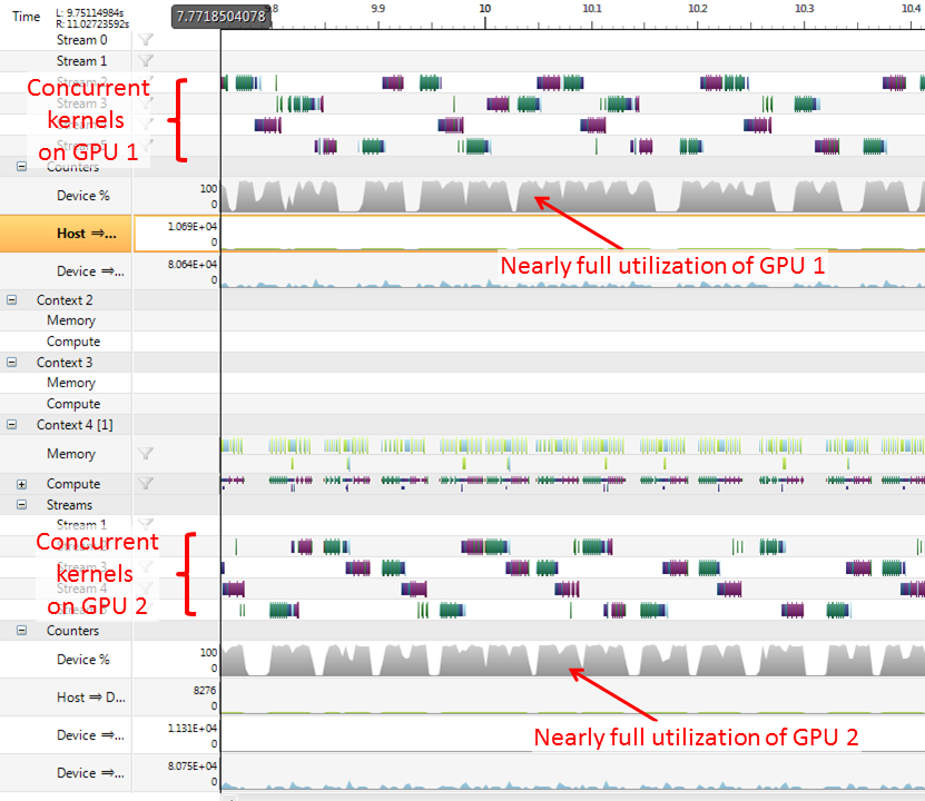
It can be seen that, despite the complex interactions on different streams, the GPUs are kept reasonably busy with these load balancing techniques.

Example

To illustrate the mapping of Quasar code onto CUDA code, we give a more elaborated example in this section. We consider a generic morphological operation, defined by the following functions:

op_min = __device__ (x,y) -> min(x,y)

function y = morph_filter[T](x : cube[T], mask : mat[T], ctr : ivec2, init : T, morph_op : [__device__ (T, T) -> T])
    function [] = __kernel__ kernel (x : cube[T]'mirror, y, mask : mat[T]'unchecked'hwconst, ctr, init, morph_op, pos)
        {!kernel_transform enable="localwindow"}
        res = init
        for m=0..size(mask,0)-1
            for n=0..size(mask,1)-1
                if mask[m,n] != 0
                    res = morph_op(res,x[pos+[m-ctr[0],n-ctr[1],0]])
                endif
            endfor
        endfor
        y[pos] = res
    endfunction

    y = cube[T](size(x))
    parallel_do(size(x),x,y,mask,ctr,init,morph_op,kernel)
endfunction

The morphological filter is generic in the sense that the data types for the operation are not specified, and also not the operation morph_op. Initially, the code purely works in the global memory and requires several accesses to x (in practice, depending on the size of the mask).

Using the following compiler transform steps/optimizations, the above code transformed to code that makes use of the shared memory. In particular, the following steps are being performed:

specialization of the generic functions op_min and morph_filter
inlining of op_min
constancy analysis of the kernel function parameters
dependency analysis of the kernel function parameters, determining a size for the local processing window
local windowing transform, generating code using shared memory and thread synchronization.
array/matrix boundary access handling.

The resulting Quasar code is:

function [y:cube] = morph_filter(x:cube,mask:mat,ctr:ivec2,init:scalar)=static
    function [] __kernel__ kernel(x:cube'const'mirror,y:cube,mask:mat'const'unchecked'hwconst,ctr:ivec2'const,init:scalar'const,pos:ivec3,blkpos:ivec3,blkdim:ivec3)=static

        {!kernel name="kernel"; target="gpu"}
        sh$x=shared((blkdim+[((((size(mask,0)-1)-ctr[0])+ctr[0])+1),((((size(mask,1)-1)-ctr[1])+ctr[1])+1),1]))
        sh$x[blkpos]=x[(pos+[-(ctr[0]),-(ctr[1]),0])]

        if (blkpos[1]<(((size(mask,1)-1)-ctr[1])+ctr[1]))
            sh$x[(blkpos+[0,blkdim[1],0])]=x[(pos+[-(ctr[0]),-(ctr[1]),0]+[0,blkdim[1],0])]
        endif
        if (blkpos[0]<(((size(mask,0)-1)-ctr[0])+ctr[0]))
            sh$x[(blkpos+[blkdim[0],0,0])]=x[(pos+[-(ctr[0]),-(ctr[1]),0]+[blkdim[0],0,0])]
        endif       
        if ((blkpos[1]<(((size(mask,1)-1)-ctr[1])+ctr[1]))&&(blkpos[0]<(((size(mask,0)-1)-ctr[0])+ctr[0])))
            sh$x[(blkpos+[blkdim[0],blkdim[1],0])]=x[(pos+[-(ctr[0]),-(ctr[1]),0]+[blkdim[0],blkdim[1],0])]
        endif

        blkof$x=((blkpos-pos)-[-(ctr[0]),-(ctr[1]),0])
        syncthreads

        res=init
        for m=0..(size(mask,0)-1)
            for n=0..(size(mask,1)-1)
                if ($getunchk(mask,m,n)!=0)
                    res=min(res,sh$x[(pos+[(m-ctr[0]),(n-ctr[1]),0]+blkof$x)])
                endif
            endfor
        endfor
        y[pos,res]
    endfunction

    y=cube(size(x))
    parallel_do(size(x),x,y,mask,ctr,init,kernel)
endfunction

Equivalently, the user could have written this kernel function from the first time. However, many users do not prefer to do this, because 1) it requires more work, 2) it is prone to errors, 3) the code readability is reduced.

Finally, the generated kernel function can straightforwardly be translated to CUDA code.